銀行口座解約の予測

はじめに
現職でマーケターやWEBの分析を担当しており、最近は特に顧客の行動分析の需要が高まっています。
昨今のデータ量の増加と共に、手動でのデータ処理の限界を感じたため、データ分析スキルを向上させることにしました。このため、新しい知識が必要となり、Aidemy Premiumの「データ分析コース」を6ヶ月間受講しました。このコースでは、機械学習を使った効率的なデータ分析方法を学びました。完全に理解したわけではありませんが、この記事で学んだことを備忘録として記録します。
この記事を通して、皆様が機械学習に興味を持つきっかけになれば幸いです。
本記事の概要
この記事では、銀行の顧客データセットを利用して、顧客が口座を解約するかどうかを予測するモデルを構築します。分析に用いるデータセットには、顧客のID、姓、クレジットスコア、居住地、性別、年齢、勤続年数、口座残高、保有製品数、クレジットカードの有無、アクティブメンバーであるか、推定給与、そして口座解約の有無が含まれます。
本研究の目的は、顧客の特性や行動がどのように口座解約に影響を与えるかを解析し、それを基に予測モデルを作成することです。データの確認から始め、相関関係の検証、必要な前処理を行った上で、以下の機械学習モデルを用いて学習と評価を進めます。
ロジスティック回帰モデル
ランダムフォレスト
勾配ブースティング分類器
TensorFlowを用いたディープラーニングモデル
LightGBM
これらのモデルを比較し、顧客の口座解約予測に最適なモデルを選定します。
この分析は、銀行における顧客保持戦略をより効果的に立案することが期待されます。
作成したプログラム
ライブラリの読み込み
import pandas as pd
import numpy as np
import matplotlib.pyplot as plt
import seaborn as sns
from sklearn.preprocessing import LabelEncoder
from sklearn.model_selection import train_test_split
from sklearn.linear_model import LogisticRegression
from sklearn.metrics import accuracy_score,confusion_matrix,classification_report
from sklearn.preprocessing import StandardScaler
from sklearn.ensemble import RandomForestClassifier
from sklearn.ensemble import GradientBoostingClassifier
データの確認
最初の5行を表示して、データの構造を確認する
# csvの読み込み
# 最初の5行を表示して、データの構造を確認する
df = pd.read_csv('/content/drive/MyDrive/成果物/Churn_Modelling.csv')
df.head()
|index|RowNumber|CustomerId|Surname|CreditScore|Geography|Gender|Age|Tenure|Balance|NumOfProducts|HasCrCard|IsActiveMember|EstimatedSalary|Exited|
|---|---|---|---|---|---|---|---|---|---|---|---|---|---|---|
|0|1|15634602|Hargrave|619|France|Female|42|2|0.0|1|1|1|101348.88|1|
|1|2|15647311|Hill|608|Spain|Female|41|1|83807.86|1|0|1|112542.58|0|
|2|3|15619304|Onio|502|France|Female|42|8|159660.8|3|1|0|113931.57|1|
|3|4|15701354|Boni|699|France|Female|39|1|0.0|2|0|0|93826.63|0|
|4|5|15737888|Mitchell|850|Spain|Female|43|2|125510.82|1|1|1|79084.1|0|
# データフレームの形式を確認する
df.shape
(10000, 14)
# データ型の確認
df.info()
<class 'pandas.core.frame.DataFrame'>
RangeIndex: 10000 entries, 0 to 9999
Data columns (total 14 columns):
Column Non-Null Count Dtype
0 RowNumber 10000 non-null int64
1 CustomerId 10000 non-null int64
2 Surname 10000 non-null object
3 CreditScore 10000 non-null int64
4 Geography 10000 non-null object
5 Gender 10000 non-null object
6 Age 10000 non-null int64
7 Tenure 10000 non-null int64
8 Balance 10000 non-null float64
9 NumOfProducts 10000 non-null int64
10 HasCrCard 10000 non-null int64
11 IsActiveMember 10000 non-null int64
12 EstimatedSalary 10000 non-null float64
13 Exited 10000 non-null int64
dtypes: float64(2), int64(9), object(3)
memory usage: 1.1+ MB
データの前処理
# 欠損値の有無を確認
df.isna().sum()
RowNumber 0
CustomerId 0
Surname 0
CreditScore 0
Geography 0
Gender 0
Age 0
Tenure 0
Balance 0
NumOfProducts 0
HasCrCard 0
IsActiveMember 0
EstimatedSalary 0
Exited 0
dtype: int64
# LabelEncoderでobjectのデータ型を数値に変換して、元の列に置き換える
lb = LabelEncoder()
for column in df.columns:
    if df[column].dtype == 'object':
        df[column] = lb.fit_transform(df[column])
# データの確認 Geography Genderが数値データになっていることを確認
df.head()|index|RowNumber|CustomerId|Surname|CreditScore|Geography|Gender|Age|Tenure|Balance|NumOfProducts|HasCrCard|IsActiveMember|EstimatedSalary|Exited|
|---|---|---|---|---|---|---|---|---|---|---|---|---|---|---|
|0|1|15634602|1115|619|0|0|42|2|0.0|1|1|1|101348.88|1|
|1|2|15647311|1177|608|2|0|41|1|83807.86|1|0|1|112542.58|0|
|2|3|15619304|2040|502|0|0|42|8|159660.8|3|1|0|113931.57|1|
|3|4|15701354|289|699|0|0|39|1|0.0|2|0|0|93826.63|0|
|4|5|15737888|1822|850|2|0|43|2|125510.82|1|1|1|79084.1|0|
データの可視化
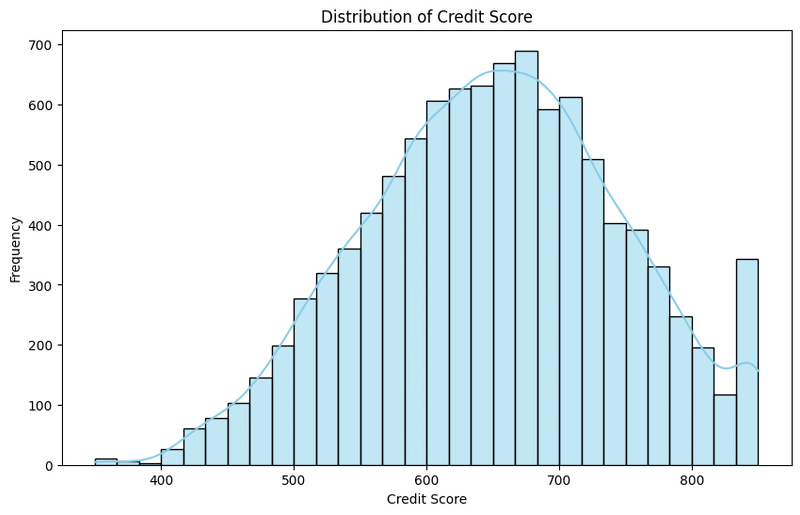
1. クレジットスコアの分布
plt.figure(figsize=(10, 6))
sns.histplot(data=df, x='CreditScore', bins=30, kde=True, color='skyblue')
plt.title('Distribution of Credit Score')
plt.xlabel('Credit Score')
plt.ylabel('Frequency')
plt.show()
600後半をピークに、山なりに分布しているが、一番最後にもう一つピークが来ている。これは、クレジットスコアの上限が850であることから、最後にピークが現れれていることが原因と考えられる
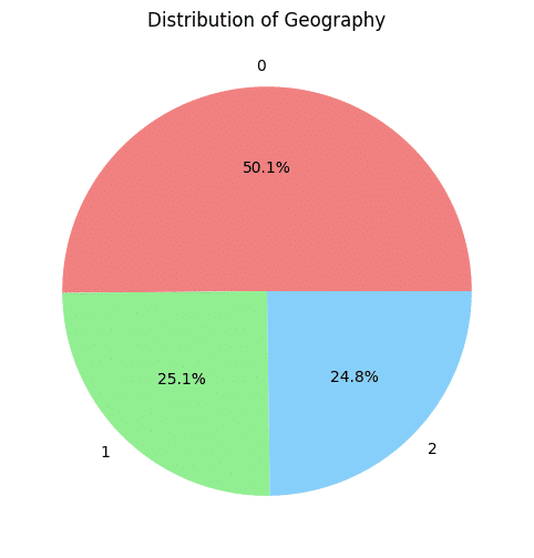
2. 居住地の割合
plt.figure(figsize=(8, 6))
df['Geography'].value_counts().plot(kind='pie', autopct='%1.1f%%', colors=['lightcoral', 'lightgreen', 'lightskyblue'])
plt.title('Distribution of Geography')
plt.ylabel('')
plt.show()
今回のデータがフランス、スペイン、ドイツのデータなので、3か国に分類される。
(何か国なのかわからない場合、バリエーション数を取って判断する必要がある)
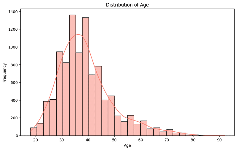
3. 年齢の分布
plt.figure(figsize=(10, 6))
sns.histplot(data=df, x='Age', bins=30, kde=True, color='salmon')
plt.title('Distribution of Age')
plt.xlabel('Age')
plt.ylabel('Frequency')
plt.show()
30代中盤をピークに広がっている
18歳からのデータになっている
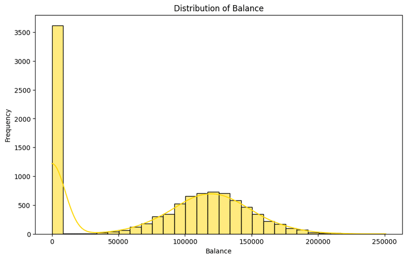
4. 預金残高の分布
plt.figure(figsize=(10, 6))
sns.histplot(data=df, x='Balance', bins=30, kde=True, color='gold')
plt.title('Distribution of Balance')
plt.xlabel('Balance')
plt.ylabel('Frequency')
plt.show()
預金残高が0の人が圧倒的に多く、残高がある人は125,000をピークになだらかに広がっている
預金残高の有無で分けたほうがよさそう
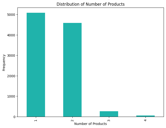
5. 利用している銀行商材の数の分布
plt.figure(figsize=(8, 6))
df['NumOfProducts'].value_counts().plot(kind='bar', color='lightseagreen')
plt.title('Distribution of Number of Products')
plt.xlabel('Number of Products')
plt.ylabel('Frequency')
plt.show()
1-2商材を契約しているユーザが多く、3以上の商材を契約しているユーザは圧倒的に少ない
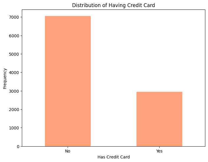
6. クレジットカード保有の比率
plt.figure(figsize=(8, 6))
df['HasCrCard'].value_counts().plot(kind='bar', color='lightsalmon')
plt.title('Distribution of Having Credit Card')
plt.xlabel('Has Credit Card')
plt.ylabel('Frequency')
plt.xticks(ticks=[0, 1], labels=['No', 'Yes'], rotation=0)
plt.show()
クレジットカードを保有していないユーザーが多い
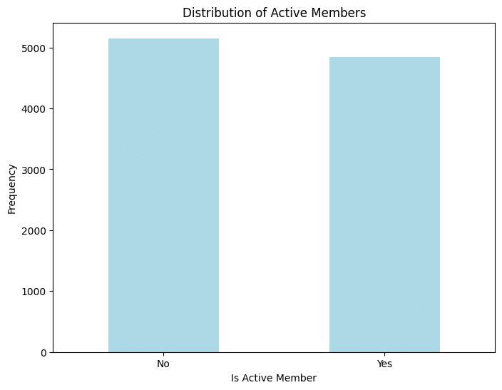
7. アクティブユーザーの比率
plt.figure(figsize=(8, 6))
df['IsActiveMember'].value_counts().plot(kind='bar', color='lightblue')
plt.title('Distribution of Active Members')
plt.xlabel('Is Active Member')
plt.ylabel('Frequency')
plt.xticks(ticks=[0, 1], labels=['No', 'Yes'], rotation=0)
plt.show()
半々くらいの割合で、アクティブ、非アクティブユーザが分布している
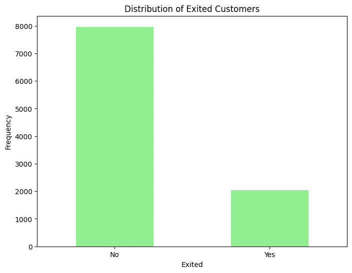
8. 銀行口座解約ユーザの比率
plt.figure(figsize=(8, 6))
df['Exited'].value_counts().plot(kind='bar', color='lightgreen')
plt.title('Distribution of Exited Customers')
plt.xlabel('Exited')
plt.ylabel('Frequency')
plt.xticks(ticks=[0, 1], labels=['No', 'Yes'], rotation=0)
plt.show()
口座解約ユーザが約2,000に対し、継続利用しているユーザは約8,000と偏った状態
データの相関関係の確認
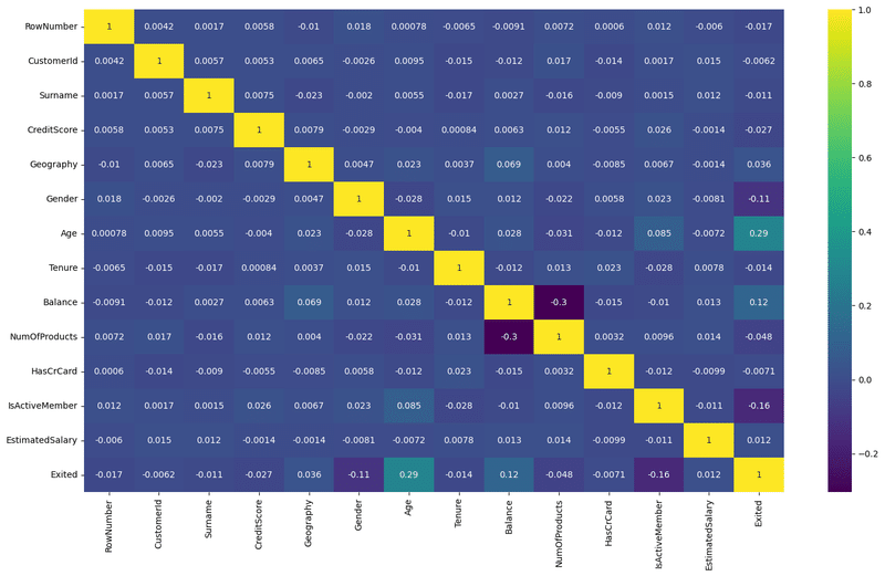
correlation = df.corr()

palette = sns.color_palette("viridis", as_cmap=True)
plt.figure(figsize=(18,10))
sns.heatmap(correlation,annot=True,cmap= palette)
plt.show()
口座解約(Exited)への相関が強いものは、
年齢
アクティブユーザー
預金残高
性別
の順番に相関していることがわかる
X = df.drop(['RowNumber','Exited'],axis=1)
Y = df['Exited']
データフレームから、行番号と解約の変数を削除して説明変数Xを作り、解約の変数だけの目的変数Yを作る
特徴量を標準化
StandardScalerで特徴量を標準化する
scaled = StandardScaler()
X_scaled = scaled.fit_transform(X)
データの分割
scikit-learnのtrain_test_splitで訓練データとテストデータを0.2で分割する
X_train,X_test,y_train,y_test = train_test_split(X_scaled,Y, test_size=0.2,random_state=42)機械学習モデル
confusion_matrixで陽性、陰性、擬陽性、偽陰性を分けて、ヒートマップで表示
classification_reportで分類指標(適合率、再現率、F1スコア)を表示
※口座を継続したユーザ・・・0 口座を解約したユーザ・・・1
ロジスティック回帰モデルでの学習と評価
口座を継続したユーザの予測はうまくいっているが、口座解約したユーザの予測はうまくいっていない
適合率:継続ユーザが0.83に対し、解約ユーザは0.62
再現率:継続ユーザが0.97に対し、解約ユーザは0.19
F1スコア:継続ユーザが0.90に対し、解約ユーザは0.29
Accuracy:0.82
# Creating and training the Logistic Regression model
model_lr = LogisticRegression()
model_lr.fit(X_train,y_train)

# Prediction on test data
y_pred = model_lr.predict(X_test)


# Evaluating the model
accuracy = accuracy_score(y_test,y_pred)
print('Model Accuracy: ',accuracy)

# Confusion_matrix:
conf_matrix = confusion_matrix(y_test,y_pred)
print("Confusion Matrix:")
print(conf_matrix)
plt.figure(figsize=(16,8))
sns.heatmap(conf_matrix,annot=True,fmt='g', cmap='Blues')
plt.xlabel('Predicted')
plt.ylabel('Actual')
plt.title('Confusion Matrix')
plt.show()
 #Classification  Report:
print("Classification Report:")
print(classification_report(y_test, y_pred, zero_division=1))
Model Accuracy: 0.8175
Confusion Matrix:
[[1561 46]
[ 319 74]
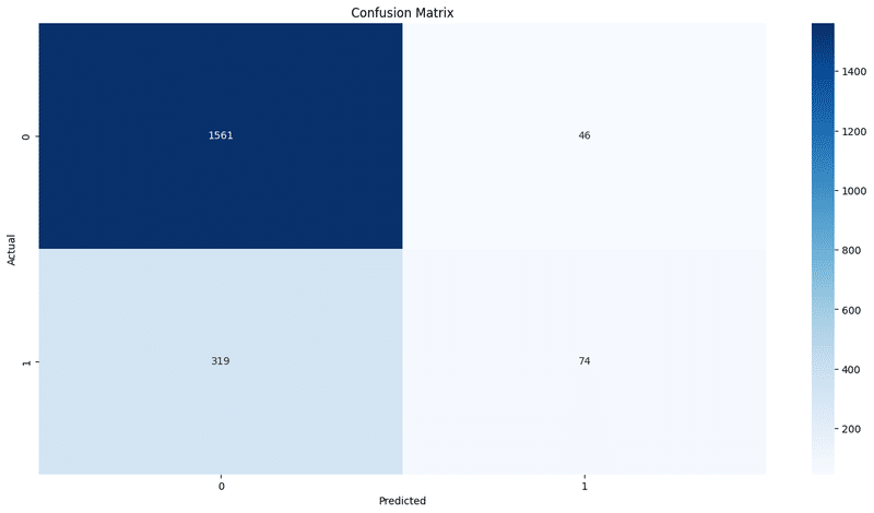
Classification Report:
precision recall f1-score support
       0       0.83      0.97      0.90      1607
       1       0.62      0.19      0.29       393

accuracy                           0.82      2000
macro avg 0.72 0.58 0.59 2000
weighted avg 0.79 0.82 0.78 2000
ランダムフォレストでの学習と評価
口座を継続したユーザの予測はうまくいっているが、口座解約したユーザの予測はややうまくいっていない
適合率:継続ユーザが0.88に対し、解約ユーザは0.76
再現率:継続ユーザが0.96に対し、解約ユーザは0.45
F1スコア:継続ユーザが0.92に対し、解約ユーザは0.56
Accuracy:0.86
# Creating and training the Logistic Regression model
model_rf = RandomForestClassifier()
model_rf.fit(X_train,y_train)

# Prediction on test data
y_pred = model_rf.predict(X_test)


# Evaluating the model
accuracy = accuracy_score(y_test,y_pred)
print('Model Accuracy: ',accuracy)

# Confusion_matrix:
conf_matrix = confusion_matrix(y_test,y_pred)
print("Confusion Matrix:")
print(conf_matrix)
plt.figure(figsize=(16,8))
sns.heatmap(conf_matrix,annot=True,fmt='g', cmap='Blues')
plt.xlabel('Predicted')
plt.ylabel('Actual')
plt.title('Confusion Matrix')
plt.show()
 #Classification  Report:
print("Classification Report:")
print(classification_report(y_test, y_pred, zero_division=1))
Model Accuracy: 0.8175
Confusion Matrix:
[[1561 46]
[ 319 74]]

Classification Report:
precision recall f1-score support
       0       0.83      0.97      0.90      1607
       1       0.62      0.19      0.29       393

accuracy                           0.82      2000
macro avg 0.72 0.58 0.59 2000
weighted avg 0.79 0.82 0.78 2000
勾配ブースティング分類器の学習と評価
口座を継続したユーザの予測はうまくいっているが、口座解約したユーザの予測はややうまくいっていない
→ランダムフォレストとほぼ同じ結果
適合率:継続ユーザが0.88に対し、解約ユーザは0.76
再現率:継続ユーザが0.96に対し、解約ユーザは0.46
F1スコア:継続ユーザが0.92に対し、解約ユーザは0.58
Accuracy:0.87
gb_model = GradientBoostingClassifier(n_estimators=100, learning_rate=0.1, random_state=42)

gb_model.fit(X_train, y_train)

# Prediction on test data
y_pred = gb_model.predict(X_test)


# Evaluating the model
accuracy = accuracy_score(y_test,y_pred)
print('Model Accuracy: ',accuracy)

# Confusion_matrix:
conf_matrix = confusion_matrix(y_test,y_pred)
print("Confusion Matrix:")
print(conf_matrix)
plt.figure(figsize=(16,8))
sns.heatmap(conf_matrix,annot=True,fmt='g', cmap='Blues')
plt.xlabel('Predicted')
plt.ylabel('Actual')
plt.title('Confusion Matrix')
plt.show()
 #Classification  Report:
print("Classification Report:")
print(classification_report(y_test, y_pred, zero_division=1))
Model Accuracy: 0.866
Confusion Matrix:
[[1550 57]
[ 211 182]]
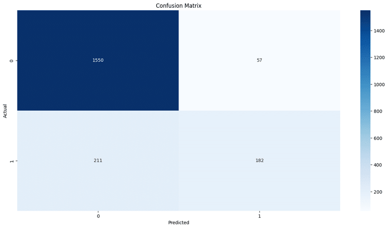
Classification Report:
precision recall f1-score support
       0       0.88      0.96      0.92      1607
       1       0.76      0.46      0.58       393

accuracy                           0.87      2000
macro avg 0.82 0.71 0.75 2000
weighted avg 0.86 0.87 0.85 2000
Tensorflow Modelの学習と評価
1エポック目では、
loss: 0.4617
accuracy: 0.8020
val_loss: 0.4177
val_accuracy: 0.8269 だったが、
5エポック目では、
loss: 0.3492
accuracy: 0.8581
val_loss: 0.3520
val_accuracy: 0.8519
と精度を改善できた。 10エポック目では、
loss: 0.3288
accuracy: 0.8631
val_loss: 0.3475
val_accuracy: 0.8481 と安定してきた
最終的にAccuracy: 0.8595となった
import tensorflow as tf

# Creating the model
model_tf = tf.keras.Sequential([
    tf.keras.layers.Dense(64, activation='relu', input_shape=(X_train.shape[1],)),
    tf.keras.layers.Dense(32, activation='relu'),
    tf.keras.layers.Dense(1, activation='sigmoid')
])

# Compiling the model
model_tf.compile(optimizer='adam',
              loss='binary_crossentropy',
              metrics=['accuracy'])

# Training the model
history = model_tf.fit(X_train, y_train, epochs=10, batch_size=32, validation_split=0.2, verbose=1)

# Testing the model
y_pred_tf = model_tf.predict(X_test)
y_pred_tf = (y_pred_tf > 0.5).astype(int)  # Converting predictions to integers based on the threshold of 0.5

# Evaluating the model
accuracy_tf = accuracy_score(y_test, y_pred_tf)
print("TensorFlow Model Accuracy:", accuracy_tf)
Epoch 1/10
200/200 [==============================] - 2s 6ms/step - loss: 0.4753 - accuracy: 0.7902 - val_loss: 0.4184 - val_accuracy: 0.8250
Epoch 2/10
200/200 [==============================] - 1s 4ms/step - loss: 0.4068 - accuracy: 0.8311 - val_loss: 0.3844 - val_accuracy: 0.8431
Epoch 3/10
200/200 [==============================] - 2s 9ms/step - loss: 0.3735 - accuracy: 0.8492 - val_loss: 0.3671 - val_accuracy: 0.8456
Epoch 4/10
200/200 [==============================] - 2s 8ms/step - loss: 0.3584 - accuracy: 0.8544 - val_loss: 0.3625 - val_accuracy: 0.8406
Epoch 5/10
200/200 [==============================] - 1s 6ms/step - loss: 0.3513 - accuracy: 0.8553 - val_loss: 0.3558 - val_accuracy: 0.8431
Epoch 6/10
200/200 [==============================] - 1s 6ms/step - loss: 0.3452 - accuracy: 0.8592 - val_loss: 0.3504 - val_accuracy: 0.8494
Epoch 7/10
200/200 [==============================] - 1s 3ms/step - loss: 0.3414 - accuracy: 0.8586 - val_loss: 0.3510 - val_accuracy: 0.8456
Epoch 8/10
200/200 [==============================] - 0s 2ms/step - loss: 0.3387 - accuracy: 0.8627 - val_loss: 0.3478 - val_accuracy: 0.8475
Epoch 9/10
200/200 [==============================] - 1s 3ms/step - loss: 0.3352 - accuracy: 0.8653 - val_loss: 0.3477 - val_accuracy: 0.8469
Epoch 10/10
200/200 [==============================] - 0s 2ms/step - loss: 0.3310 - accuracy: 0.8631 - val_loss: 0.3462 - val_accuracy: 0.8481
63/63 [==============================] - 0s 1ms/step
TensorFlow Model Accuracy: 0.863
ロジスティック回帰モデル
精度: 0.82
ランダムフォレスト
精度: 0.86
勾配ブースティング
精度: 0.87
TensorFlow Model
精度: 0.8595
今のところ、勾配ブースティングが最も予測精度が高いモデルだったといえる。
データの前処理の追加
以下のデータの前処理を追加し、精度を高める
クレジットスコアが850を超えている人を1、そのほかを0にする
預金残高が0の人を1、そのほかを0にする
銀行商材が1の人を1、2以上の人を0にする
df['isCreditScoreMax'] = 0 #
df.loc[df['CreditScore'] == 850, 'isCreditScoreMax'] = 1

df['isBalanceZero'] = 0 #
df.loc[df['Balance'] == 0, 'isBalanceZero'] = 1

df['isNumOfProductsSingle'] = 0 #
df.loc[df['NumOfProducts'] == 1, 'isNumOfProductsSingle'] = 1

df.head()
|index|RowNumber|CustomerId|Surname|CreditScore|Geography|Gender|Age|Tenure|Balance|NumOfProducts|HasCrCard|IsActiveMember|EstimatedSalary|Exited|isCreditScoreMax|isBalanceZero|isNumOfProductsSingle|
|---|---|---|---|---|---|---|---|---|---|---|---|---|---|---|---|---|---|
|0|1|15634602|1115|619|0|0|42|2|0\.0|1|1|1|101348\.88|1|0|1|1|
|1|2|15647311|1177|608|2|0|41|1|83807\.86|1|0|1|112542\.58|0|0|0|1|
|2|3|15619304|2040|502|0|0|42|8|159660\.8|3|1|0|113931\.57|1|0|0|0|
|3|4|15701354|289|699|0|0|39|1|0\.0|2|0|0|93826\.63|0|0|1|0|
|4|5|15737888|1822|850|2|0|43|2|125510\.82|1|1|1|79084\.1|0|1|0|1|
# データフレームから、行番号と解約の変数を削除して説明変数Xを作り、解約の変数だけの目的変数Yを作る
X = df.drop(['RowNumber','Exited'],axis=1)
Y = df['Exited']

# scikit-learnのtrain_test_splitで訓練データとテストデータを0.2で分割する
# Splitting data into train and test sets
X_train,X_test,y_train,y_test = train_test_split(X,Y, test_size=0.2,random_state=42)
モデルの追加
lightGBMでモデルの学習を行う
import lightgbm as lgb


lgb_params = {
    "objective": "regression",
    "metric": "rmse",
    "random_state": 42
}

train_lgb = lgb.Dataset(X_train, y_train)

model = lgb.train(
    lgb_params,
    train_lgb,
    num_boost_round=1000,
    )

# 特徴量重要度の表を作成
importance_df = pd.DataFrame({
    "feature_names":model.feature_name(),
    "importances":model.feature_importance("gain")
})
display(importance_df.sort_values("importances", ascending=False).head(12))

accuracy_tf = accuracy_score(y_test, y_pred_tf)
print("TensorFlow Model Accuracy:", accuracy_tf)
[LightGBM] [Info] Auto-choosing row-wise multi-threading, the overhead of testing was 0.000918 seconds.
You can set `force_row_wise=true` to remove the overhead.
And if memory is not enough, you can set `force_col_wise=true`.
[LightGBM] [Info] Total Bins 1372
[LightGBM] [Info] Number of data points in the train set: 8000, number of used features: 15
[LightGBM] [Info] Start training from score 0.205500
|index|feature_names|importances|
|---|---|---|
|5|Age|1495.5129171857843|
|8|NumOfProducts|930.0853415811434|
|7|Balance|792.424500106601|
|11|EstimatedSalary|572.1997283796081|
|0|CustomerId|559.883876038366|
|2|CreditScore|555.7048681692104|
|1|Surname|549.4598454960505|
|10|IsActiveMember|444.44999793329043|
|3|Geography|243.3842243622057|
|6|Tenure|242.48473496118095|
|4|Gender|104.18366198113654|
|9|HasCrCard|43.48622356378473|
TensorFlow Model Accuracy: 0.863
y_pred = model.predict(X_test)
test_acc = accuracy_score(
    y_test, np.where(y_pred>=0.5, 1, 0)
    )
print(test_acc)
0.8605
gb_model = GradientBoostingClassifier(n_estimators=100, learning_rate=0.1, random_state=42)

gb_model.fit(X_train, y_train)

# Prediction on test data
y_pred = gb_model.predict(X_test)


# Evaluating the model
accuracy = accuracy_score(y_test,y_pred)
print('Model Accuracy: ',accuracy)

# Confusion_matrix:
conf_matrix = confusion_matrix(y_test,y_pred)
print("Confusion Matrix:")
print(conf_matrix)
plt.figure(figsize=(16,8))
sns.heatmap(conf_matrix,annot=True,fmt='g', cmap='Blues')
plt.xlabel('Predicted')
plt.ylabel('Actual')
plt.title('Confusion Matrix')
plt.show()
 #Classification  Report:
print("Classification Report:")
print(classification_report(y_test, y_pred, zero_division=1))
Model Accuracy: 0.867
Confusion Matrix:
[[1550 57]
[ 209 184]]
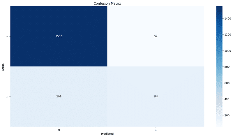
Classification Report:
precision recall f1-score support
       0       0.88      0.96      0.92      1607
       1       0.76      0.47      0.58       393

accuracy                           0.87      2000
macro avg 0.82 0.72 0.75 2000
weighted avg 0.86 0.87 0.85 2000
結果
勾配ブースティングが最も予測精度が高いモデルだった
前処理を追加したデータフレームで、先の4モデルでも検証を行ったが、ほとんど精度の向上はなかった
今後の活用
このモデルを活用すれば、銀行はどの顧客が口座を解約するか予測できるようになります。これにより、リスクの高い顧客に対してパーソナライズされたキャンペーンやサービス改善の対応を行い、顧客の満足度を高めることが可能となり、口座の解約率を抑えることが期待できます。
おわりに
この記事では、Pythonと機械学習を使って銀行口座の解約予測モデルを構築する過程を、自分自身の学習の記録として共有しました。
私自身、まだ機械学習の初心者であり、実際のプロジェクトを通じて学んだことをアウトプットすることで理解を深めていきたいと考えています。
この取り組みが、同じように学びたいと思っている方々にも、何かのヒントや動機付けになれば幸いです。
これからも続けて学び、経験を積んでいきたいと思います。
この記事が気に入ったらサポートをしてみませんか?