Aaron Bramson, Ph.D.

Introduction

Residential demand estimation is important for setting rent and sales prices, predicting vacancy risk, identifying areas underserviced or overserviced by transportation resources, establishing proper zoning, determining appropriate/optimal land usage, as well as other economic and policy related decisions.  Demand for a residential unit depends on a combination of property features, building features, neighborhood features, and wider accessibility features.  Our focus here is on those wider accessibility features that require sophisticated analyses combining geospatial and network data.  

We propose a method for estimating residential property demand originating from places of employment as a way to measure the desirability of a location as a quantitative variable rather than the typical categorical geospatial variables for improving (among other things) hedonic pricing models.  Our approach calculates demand as the time-weighted potential flow of people from places of work, across the detailed multimodal transportation network, to each location in the greater Tokyo area.  

A preliminary study revealed that rent prices have a -0.714 Pearson correlation with the time to reach Tokyo Station, and the log prices have a -0.74 correlation.  The concentration of jobs in that region (rather than other sources of demand) lead us to examine an employment-based demand hypothesis more deeply. The convenience of a location to reach a large number of jobs is intuitively linked to that location’s value, and this work aims to precisely quantify that connection.

Methods

Here we describe our methodology divided into three topics: our data, our network construction, and our approach to estimating demand using network propagation.

Data

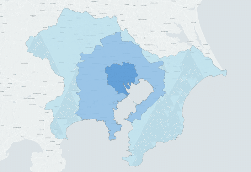
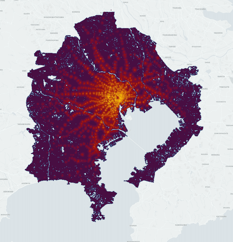
Our region of analysis is the Tokyo Main Metropolitan Area; a custom region roughly following the E16 circuit road designed to include only those regions relevant to commuting within Tokyo as shown in Figure 1.  It covers 36% of the land area of the Greater Tokyo Area (prefectures of Tokyo, Saitama, Kanagawa and Chiba), but includes 92% of its population.  The region covered has a population of 32,197,448, 15,080,305 salaried jobs, and a surface area of 4,893 km2.

Our walking network data comes from Open Street Map (OSM). We filter the OSM “road” network to edges where walking is possible and permitted.  Nodes for station exits are already connected to the road network (after some manual OSM data cleaning).  We connect station nodes to all exit nodes within 250m with access links having an approximate walking time.  The 1,440 station nodes also exist within our train network built from OSM and Wikipedia data.  By merging the walking and train networks, we have a high fidelity system for determining the traversal times between any two points within the sizable Tokyo Main Area.  However, because the geographic area is so large, it is impractical to calculate long-distance traversals on the walking network directly.  Instead, we need to create a simplified geospatial network with approximate (but accurate) traversal times to use as a proxy for the walking network.

Geospatial Hex Network

We first create a 250m inner diameter hexagonal grid covering the area, excluding hexes that contain no road segments.  Each of the 137,221 hexes are connected to the walking network by creating a hex access link between the hex centroid and the closest point on the walking network (edge or node).  Hex nodes are also connected to station nodes within 375m.  Then hexes are connected to all neighboring hexes; in one set of experiments only immediate neighbors are connected, and in another set of experiments we expand to radius-2 neighbors (within 510m).  The walking times for hex-hex and hex-station connections have edge weights calculated as the traversal time across the walking network. Hex-hex edges requiring more than 30 minutes, and hex-station edges requiring more than 15 minutes, are removed, then all the road edges are removed from the network leaving the hex+train network.  In this way we maintain highly accurate traversal times (and include only walkable routes) while greatly reducing the number of edges to make the problem tractable.  

Demand Analysis

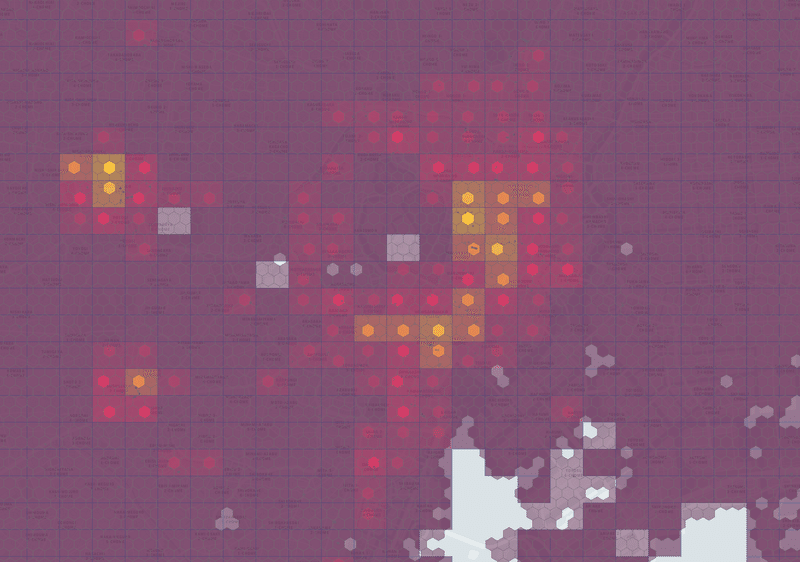
The hexes of the network also serve as intuitive units to hold quantities relevant to our analysis and to visualize the data and results.  We assign source demand from 500m square grid data of the number of salaried employees to the hex which overlaps the grid's centroid, resulting in 17,201 hexes with source flow.  By far the strongest concentration of jobs is the downtown area surrounding Tokyo, Nihonbashi, and Otemachi stations (see Figure 2); however, a non-negligible number of jobs exist in secondary city centers (e.g. Shinjuku, Shibuya, Yokohama).

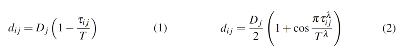
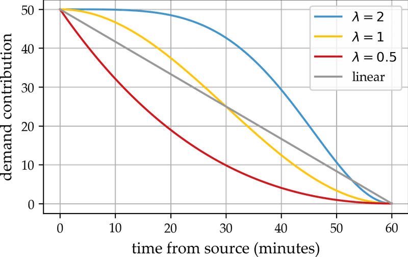
From each source hex node, we propagate the demand across the integrated hex+train network using eight time-weighting discount functions to evaluate the combined demand from all sources at each hex.  As a baseline, we estimate the demand contribution dij at hex i from source j with source flow value Dj using the linear function in Equation 1 where 𝜏ij is the traversal time from hex i to hex j and T∈{60, 90} is the time horizon for the diffusion process.  We also examine parameterized nonlinear discounting relationships using Equation 2 with  λ∈{0.5, 1.0, 2.0} to capture different levels of sensitivity to traversal times. A plot of these functions using an example of 50 source jobs and a time horizon of 60 minutes appears in Figure 3.  The total demand for hex i is the sum of the time-discounted demand from all sources: Σj dij.

Results

The raw results are the distributions of projected demand from the job sources across the hex grid based on each version of the weighting function.  You can see the result for linear discounting over a 90 minute horizon in Figure 4.  The distributions are qualitatively similar for all discount functions, and are quantitatively different in expected ways.  The high concentration of jobs in the city center leaves a clear mark on the distribution: hexes with stations closer to downtown have greater demand and greater walking distances from stations show a clearly visible diffusion pattern.  Although the resulting estimated demand distributions are robust and intuitive, we also need a way to differentiate among parameterizations, evaluate their accuracy, and convert them into useful units for applications. 

In order to evaluate these results, we compare the estimated demand values with rental prices across the area.  First, we filter the full set of available rental properties from our database to reduce the heterogeneity in unit features.  We only include properties (1) with prices published between January 1, 2022 and July, 30 2023; (2) built within the years 2010 and 2014; (3) and sizes between 25-28m2 (one room apartments).  We find 356,744 units of similar size and age with recent prices focused on 8,413 (~6.65%) of the hexes.  This allows us to determine the correlation between our estimated demand and the value of properties. Table 1 shows the Pearson correlations between our estimated demand and rental prices using the radius-2 hex network.  The radius-1 hex network produces slightly lower values with a similar pattern.  

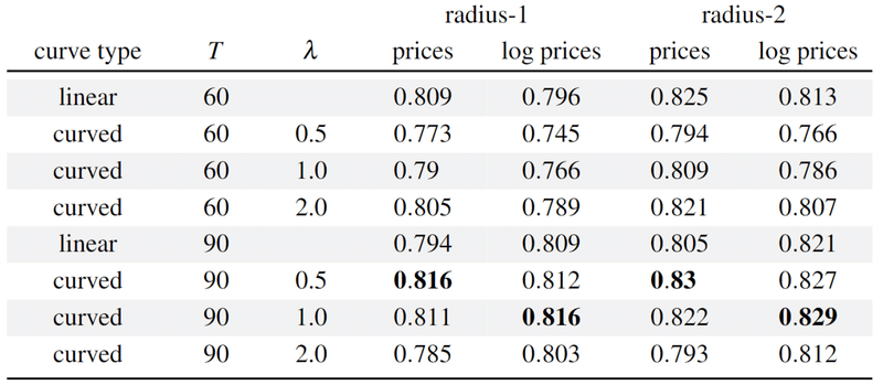
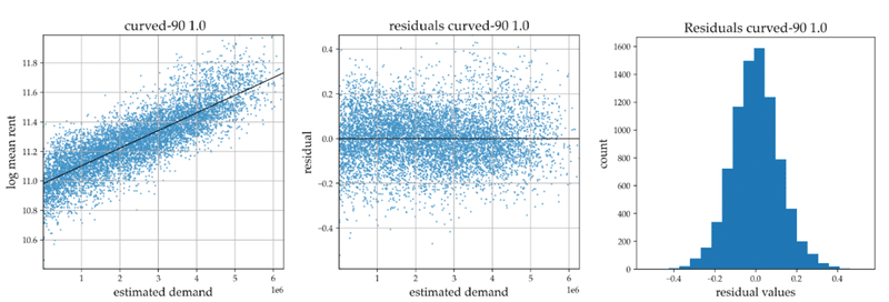
Using curved (λ=1.0, T=90) discounting, not only is the correlation a high 0.829, the pattern of the residual errors from the log price prediction are close to normally distributed and lack a distinct pattern as shown in Figure 4.  Residuals for other weighting functions, even with similar correlation values, exhibit clear non-random patterns and more skewed distribution.  With this in mind, we have selected this weighting for incorporating estimated demand into larger hedonic pricing models.

Conclusions and Future Work

Although there isn't a direct relationship between pure demand and prices (i.e., without accounting for supply limitations and asset variations), we demonstrate a partial validation by discovering that more than 80% of the variation in property prices can be explained by their distance to places of salaried employment. In addition to the high correlation values, the residuals of the errors are nicely normally distributed around the best fit line, indicating that the remaining variation in prices may be cleanly explainable by the more specific features in a detailed hedonic pricing model.

These values are already probably near the limit of how much price variation can be explained in terms of estimated demand from jobs, but we have a few refinements planned to further improve our specific estimates. Further improvements to network traversal time accuracy (e.g., incorporating slopes and additional modes and preferences of travel) may further improve the results. We also need to incorporate additional sources of demand (e.g. schools, stores, sports facilities).  We will then use the estimated demand as the base for hedonic pricing models of property valuation and determine whether they are substantially improved over existing models that lack the integrated geospatial network information.