ブレセンハムのアルゴリズム

ある理想の直線が存在するとして、それをピクセル単位に分割された、離散化されたディスプレイ空間に適切に、自然に割り当てるにはどうしたらよいか。
ブレセンハムのアルゴリズムが特筆すべきはすべてが整数演算であること。
描画したい直線が$${y=ax+b}$$であって、$${m=\frac{\Delta y}{\Delta x}}$$として除算を許容するならDDA(Digital differential analyzer)と称される。
また、ブレセンハム先生の元の論文はプロッターの動作について論じているので、コンピューターグラフィックスにおけるディスプレイ空間とはちょっと話がずれる。具体的には0.5ずれる。
プロッターはグリッドの交点に点をうつが、コンピューターグラフィックスはグリッドの交点の右下のセルを塗りつぶす。
なのでwikipediaと並行して読むと係数がずっとずれてるので頭がハテナになる。
ここでは先にブレセンハム先生の論文を見てから0.5のずれを直す。
Algorithm for computer control of a digital plotter
Bresenham, J. E. (1 January 1965). “Algorithm for computer control of a digital plotter”. IBM Systems Journal 4 (1): 25–30. doi:10.1147/sj.41.0025.
描画したい直線を第一象限、かつ0度から45度の角度に限定して考える。これを第一オクタント、八分円の最初のエリアと考える。
こうすることで我々はxを+1する毎にyを+0するか+1するかだけ考えればよくなる。xはforなりwhileなりでループするとして、我々はどのような条件でyを+1し、どのような条件で+1しないのか。
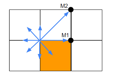
コンピューターグラフィックスにおいては通常y+の方向が反転するので注意を要する。
論文中のMなんちゃらは全部プロッターの軌道。プロッターはM1やM2のようなグリッドの交点に点をうち、CGは橙のエリアのように、交点の右下を塗りつぶす。
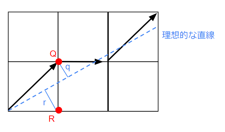
基本的な原理として、下図中の青い点線を理想の直線とするなら、
q<rであるから次の点はRでなくQを選択すべきである。
と、論文では言っている。が、繰り返すがこれはプロッターの動作、経路であってプログラム的なグラフィックスはちょっと意味が変わる。繰り返すが反転している上に半分ズレている。
それというのもブレセンハム先生のプロッターはRやQの点にそのまま点を打てばよいが、コンピューターグラフィックスの場合、座標Rを選択するということは下図においてRを左上とするピクセルを塗りつぶすということであるから、下図においては画面外を塗ることになる。この辺りはあとで半分ずらすが、今は論文を読むことに焦点を当てているため論文が述べていることを説明するにとどめる。
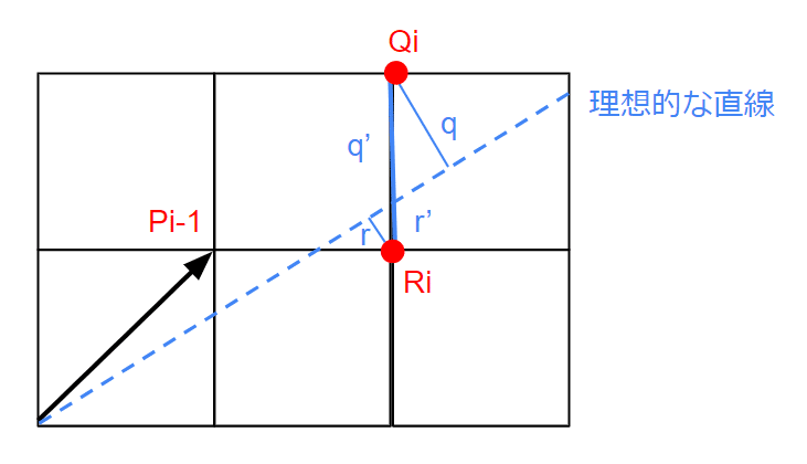
プロットが$${p_{i-1}}$$まで進んだとしよう。
次の選択肢は$${Q_i}$$か$${R_i}$$である。
$${r_i < q_i}$$もしくは$${r'_i < q'_i}$$なら次の選択肢は$${R_i}$$であろう。$${r_i ≥ q_i}$$もしくは$${r'_i ≥ q'_i}$$なら次の選択肢は$${Q_i}$$である。
現状第1象限(特にブレセンハム先生は45度以内の範囲を第1オクタント(八分円の最初)としている)の話である。
$${r'_i-q'_i}$$の符号と$${r_i-q_i}$$の符号は常に同じである。
※ここで符号を気にしているのは、比較演算$${r_i < q_i}$$は$${r_i - q_i< 0}$$にしてもやってること同じだよねという話である。ここで丁度境界上の場合どうするかは実装者の手に委ねられる。
$${D_1=(x_1,y_1), D_2=(x_2, y_2)}$$
$${(\Delta a, \Delta b)=(x_2-x_1, y_2-y_1)}$$
とすると
第一オクタントは常に$${\Delta a>0}$$であるから
$${\nabla_i=(r'_i-q'_i)\Delta a}$$も$${r_i-q_i}$$と符号が同じ。
これにより、$${\nabla_i=(r'_i-q'_i)\Delta a}$$をy+0かy+1かの選択の基準とすることができる。
つまり$${\nabla_i<0}$$か$${\nabla_i\geq0}$$によってy+0かy+1か決定しても良いということである。
$${\nabla_i}$$の更新のために
$$
\nabla_1 = 2\Delta b-\Delta a\\
\nabla_{i+1} = \begin{cases} \nabla_i +2\Delta b-2\Delta a & (\nabla_i\geq 0)
\\ \nabla_i +2\Delta b & (\nabla_i<0) \end{cases}
$$
という式が成立し、これをアルゴリズムに落とし込めば完成である。
ではこの式はどのようにして導かれるか。
ブレセンハムのアルゴリズムは、基本的にx++ごとに理想の直線と、実際にプロットに用いるy座標との誤差を累積していって、閾値を超えたら誤差から規定値を減算するということを繰り返す。
この辺はむしろウィキペディアなどの方が詳しい。
誤差とは例えば
始点と終点が$${D_1=(x_1,y_1), D_2=(x_2, y_2)}$$とあった時の
$${(\Delta a, \Delta b)=(x_2-x_1, y_2-y_1)}$$に対する
$${\frac{\Delta b}{\Delta a}}$$、すなわち直線の傾きと、実際にプロットされたy座標(整数値)との差である。
誤差が例えば0.5を超えたら1減算するとするなら、誤差は常に±0.5に収まる。つまり±0.5の範囲内で理想の直線の付近をうろちょろできる。
ここで傾きの除算だの、0.5だのを消すために数式を操作すると前述の式になったりするという解釈もできるわけだが、ここは少し我慢して先に進もう。
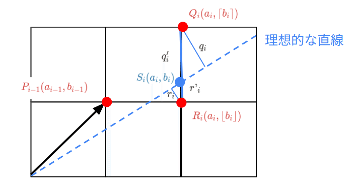
$${S_i(a_i, b_i)}$$は現在の理想直線上の座標。
$${P_{i-1}=(a_{i-1}, \hat b_{i-1})}$$はプロットした一個前の座標。
ハットがつくのはおそらく整数値に丸められているからで、理想直線上の$${b_{i-1}}$$と区別するためであろう。ただし$${b_{i-1}}$$は計算にでてこない。
我々はこれらの座標$${P_{i-1}, S{i}}$$から次にプロットする座標候補
$$
R_1(a_i, \lfloor b_i\rfloor)\\
Q_1(a_i, \lceil b_i \rceil)
$$
から1つを選択したい。
$${S_i(a_i,b_i)}$$は理想直線のあるx地点$${a_i}$$での座標である。
今、天井関数と床関数により、$${R_1}$$と$${Q_1}$$は理想直線の直下ないし直上の整数座標である。つまりプロッターが次にプロットしたいのはそのどちらかである。
$${\nabla_i=(r'_i-q'_i)\Delta a}$$が書き直されて
$${r'_i=b_i-\lfloor b_i\rfloor}$$
$${q'_i=\lceil b_i \rceil-b_i}$$
であるから
$${\nabla_i=[(b_i-\lfloor b_i\rfloor)-(\lceil b_i \rceil-b_i)]\Delta a}$$となる。
ここで$${S_i(a_i, b_i)}$$のy値は傾き$${\frac{\Delta b}{\Delta a}}$$を用いて
$$
b_i=\frac{\Delta b}{\Delta a}a_i
$$
である。つまり$${S_i(a_i, \frac{\Delta b}{\Delta a}a_i)}$$
これを$${\nabla_i=[(b_i-\lfloor b_i\rfloor)-(\lceil b_i \rceil-b_i)]\Delta a}$$に代入すると
$$
\nabla_i=[(\frac{\Delta b}{\Delta a}a_i-\lfloor b_i\rfloor)-(\lceil b_i \rceil-\frac{\Delta b}{\Delta a}a_i)]\Delta a\\
\nabla_i=\Delta a(\frac{\Delta b}{\Delta a}a_i-\lfloor b_i\rfloor)-\Delta a(\lceil b_i \rceil-\frac{\Delta b}{\Delta a}a_i)\\
\nabla_i=\frac{\Delta b}{\Delta a}a_i\Delta a-\lfloor b_i\rfloor\Delta a-\lceil b_i \rceil\Delta a+\frac{\Delta b}{\Delta a}a_i\Delta a\\
\nabla_i=2\frac{\Delta b}{\Delta a}\Delta aa_i-(\lfloor b_i\rfloor+\lceil b_i \rceil)\Delta a\\
\nabla_i=2a_i\Delta b -(\lfloor b_i\rfloor+\lceil b_i \rceil)\Delta a\\
$$
さて、第1オクタントにおいて
$$
a_i=a_{i-1}+1
$$
である。
これはx+=1みたいなことしか言ってない。
$$
\lceil b_i \rceil=\hat b_{i-1}+1\\
\lfloor b_i\rfloor=\hat b_{i-1}
$$
である。
これはx+=1した時にy+=1するかしないかみたいなことしか言ってない。
これらを式に戻すと
$$
\nabla_i=2a_i\Delta b -(\lfloor b_i\rfloor+\lceil b_i \rceil)\Delta a\\
\nabla_i=2(a_{i-1}+1)\Delta b -(\hat b_{i-1}+b_{i-1}+1)\Delta a\\
\nabla_i=2a_{i-1}\Delta b-2\hat b_{i-1}\Delta a+2\Delta b-\Delta a
$$
これで一個前の整数座標からy+=1するかしないかの基準値を求める式ができた。
初期値を$${a_0=0}$$, $${\hat b_0=0}$$とすると、
最初の$${\nabla_i}$$こと$${\nabla_1}$$は
$${\nabla_i=2a_{i-1}\Delta b-2\hat b_{i-1}\Delta a+2\Delta b-\Delta a}$$のうち最初の2項が0で消えるから
$$
\nabla_1 = 2\Delta b-\Delta a\\
$$
ここで$${\nabla_i\geq 0}$$ならば$${\hat b_i = \hat b_{i-1}+1\\}$$であるから
$$
\nabla_i=2a_{i-1}\Delta b-2\hat b_{i-1}\Delta a+2\Delta b-\Delta a\\
\nabla_{i+1}=2(a_{i-1}+1)\Delta b-2(\hat b_{i-1}+1)\Delta a+2\Delta b-\Delta a\\
\nabla_{i+1}=2a_{i-1}\Delta b+2\Delta b-2\hat b_{i-1}\Delta a -2\Delta a+2\Delta b-\Delta a\\
\nabla_{i+1} = \nabla_i +2\Delta b-2\Delta a
$$
$${\nabla_i< 0}$$ならば$${\hat b_i = \hat b_{i-1}\\}$$であるから
$$
\nabla_i=2a_{i-1}\Delta b-2\hat b_{i-1}\Delta a+2\Delta b-\Delta a\\
\nabla_{i+1}=2(a_{i-1}+1)\Delta b-2\hat b_{i-1}\Delta a+2\Delta b-\Delta a\\
\nabla_{i+1}=2a_{i-1}\Delta b+2\Delta b-2\hat b_{i-1}\Delta a +2\Delta b-\Delta a\\
\nabla_{i+1}=\nabla_i +2\Delta b
$$
あとは8象限分つくれーいとなってブレセンハム先生の論文は終わる。
半分ずらす
$${\nabla_i=(r'_i-q'_i)\Delta a}$$と
$${\nabla_i=[(b_i-\lfloor b_i\rfloor)-(\lceil b_i \rceil-b_i)]\Delta a}$$
の部分が、
$${\nabla_i=[(b_i-(\lfloor b_i\rfloor + 0.5))-((\lceil b_i \rceil+0.5)-b_i)]\Delta a}$$
$$
\nabla_i=2a_i\Delta b -(\lfloor b_i\rfloor+\lceil b_i \rceil)\Delta a-\Delta a\\
\nabla_i=2(a_{i-1}+1)\Delta b -(\hat b_{i-1}+b_{i-1}+1)\Delta a-\Delta a\\
\nabla_i=2a_{i-1}\Delta b-2\hat b_{i-1}\Delta a+2\Delta b-2\Delta a\\
\nabla_i=a_{i-1}\Delta b-\hat b_{i-1}\Delta a+\Delta b-\Delta a
$$
ここで$${\nabla_i\geq 0}$$ならば$${\hat b_i = \hat b_{i-1}+1\\}$$であるから
$$
\nabla_i=a_{i-1}\Delta b-\hat b_{i-1}\Delta a+\Delta b-\Delta a\\
\nabla_{i+1}=(a_{i-1}+1)\Delta b-(\hat b_{i-1}+1)\Delta a+\Delta b-\Delta a\\
\nabla_{i+1}=a_{i-1}\Delta b+\Delta b-\hat b_{i-1}\Delta a -\Delta a+\Delta b-\Delta a\\
\nabla_{i+1} = \nabla_i +\Delta b-\Delta a
$$
$${\nabla_i< 0}$$ならば$${\hat b_i = \hat b_{i-1}\\}$$であるから
$$
\nabla_i=a_{i-1}\Delta b-\hat b_{i-1}\Delta a+\Delta b-\Delta a\\
\nabla_{i+1}=(a_{i-1}+1)\Delta b-\hat b_{i-1}\Delta a+\Delta b-\Delta a\\
\nabla_{i+1}=a_{i-1}\Delta b+\Delta b-\hat b_{i-1}\Delta a +\Delta b-\Delta a\\
\nabla_{i+1}=\nabla_i +\Delta b
$$
コード
大丈夫かどうか不明。
第一オクタント分
def bresenham_line(x1, y1, x2, y2):
"""
Bresenham's Line Algorithm Implementation for the first octant.
This function will only work for lines in the first octant,
that is for lines with an angle between 0 and 45 degrees to the x-axis.
"""
# Calculate deltas
delta_a = x2 - x1
delta_b = y2 - y1
# Initial decision parameter
nabla_i = 2 * delta_b - delta_a
# Starting points
a = x1
b = y1
# List of points on the line
line_points = [(a, b)]
# Loop through the x range from the start to end point
while a < x2:
# Increment x
a += 1
if nabla_i >= 0:
# Increment y and update decision parameter for y + 1
b += 1
nabla_i += 2 * delta_b - 2 * delta_a
else:
# Keep y and update decision parameter for y + 0
nabla_i += 2 * delta_b
# Append the point to the list
line_points.append((a, b))
return line_points
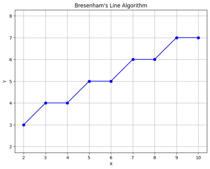
# Example usage:
# Draw line from (2,3) to (10,7), this line is in the first octant
bresenham_line(2, 3, 10, 7)# Let's define the Bresenham's line algorithm correctly to work with integer arithmetic only.
def bresenham_line(x1, y1, x2, y2):
"""
Bresenham's Line Algorithm Implementation for the first octant.
This function will only work for lines in the first octant,
that is for lines with an angle between 0 and 45 degrees to the x-axis.
"""
# Calculate deltas and steps
delta_x = x2 - x1
delta_y = y2 - y1
step_x = 1 if delta_x > 0 else -1
step_y = 1 if delta_y > 0 else -1
delta_x = abs(delta_x)
delta_y = abs(delta_y)
# Initial decision parameter
nabla_i = 2 * delta_y - delta_x
# Starting points
x, y = x1, y1
# List of points on the line
line_points = [(x, y)]
# Loop through the x range from the start to end point
while x != x2:
# Increment x
x += step_x
if nabla_i >= 0:
# Increment y and update decision parameter for y + 1
y += step_y
nabla_i -= 2 * delta_x
# Update decision parameter for y + 0
nabla_i += 2 * delta_y
# Append the point to the list
line_points.append((x, y))
return line_points
# Function to plot the points
def plot_line(points):
# Unpack points
x_points, y_points = zip(*points)
plt.figure(figsize=(8, 6))
plt.plot(x_points, y_points, 'bo-') # blue color, circle marker, solid line style
plt.title("Bresenham's Line Algorithm")
plt.xlabel("X")
plt.ylabel("Y")
plt.grid(True)
plt.axis('equal')
plt.show()
# Use the Bresenham's algorithm function to get the line points and plot the line
line_points = bresenham_line(2, 3, 10, 7)
plot_line(line_points)
表示機能を塗りつぶしに
# Correct the error by using the values directly from the line_points for setting the plot limits

def plot_bresenham_line_filled_squares_corrected(line_points):
    # Create a new figure
    fig, ax = plt.subplots(figsize=(8, 6))

    # Get min and max values for setting limits
    x_values, y_values = zip(*line_points)
    min_x, max_x = min(x_values), max(x_values)
    min_y, max_y = min(y_values), max(y_values)

    # Plot each point as a square
    for x, y in line_points:
        # Draw a filled square for each point at the top-left corner of the grid cell
        square = plt.Rectangle((x, y), 1, 1, color="blue")
        ax.add_patch(square)

    # Set the limits of the plot a bit larger than the min and max values
    ax.set_xlim([min_x - 1, max_x + 1])
    ax.set_ylim([min_y - 1, max_y + 1])

    # Add grid and set aspect ratio to equal for correct square display
    plt.grid(True)
    ax.set_aspect('equal')
    plt.title("Bresenham's Line Algorithm with Filled Squares")
    plt.xlabel("X")
    plt.ylabel("Y")

    # Show the plot
    plt.show()

# Plot the line with the correct filled squares representation
plot_bresenham_line_filled_squares_corrected(line_points)

p5.js
function setup() {
  createCanvas(400, 400);
  background(0); // Set background to black
}

function draw() {
  stroke(255); // Set stroke color to white for visibility
  let points = bresenhamLine(2, 3, 10, 7); // Draw line from (2, 3) to (10, 7)
  points.forEach((p) => {
    point(p[0], p[1]); // Ensure this uses the p5.js point() function
  });
  noLoop(); // Stops the draw loop after rendering
}

function bresenhamLine(x1, y1, x2, y2) {
  // Calculate deltas
  let deltaA = x2 - x1;
  let deltaB = y2 - y1;

  // Initial decision parameter
  let nablaI = 2 * deltaB - deltaA;

  // Starting points
  let a = x1;
  let b = y1;

  // List of points on the line
  let linePoints = [[a, b]];

  // Loop through the x range from the start to end point
  while (a < x2) {
    a += 1;
    if (nablaI >= 0) {
      b += 1;
      nablaI += 2 * deltaB - 2 * deltaA;
    } else {
      nablaI += 2 * deltaB;
    }
    linePoints.push([a, b]);
  }

  return linePoints;
}
八象限分
def bresenham_line_all_octants(x1, y1, x2, y2):
    """
    Bresenham's Line Algorithm Implementation for all octants.
    """
    # Determine differences and step directions
    delta_x = x2 - x1
    delta_y = y2 - y1
    step_x = 1 if delta_x >= 0 else -1
    step_y = 1 if delta_y >= 0 else -1
    delta_x = abs(delta_x)
    delta_y = abs(delta_y)

    # Initialize starting points and decision variable
    x, y = x1, y1
    nabla_i = 2 * delta_y - delta_x if delta_x >= delta_y else 2 * delta_x - delta_y

    # List of points on the line
    line_points = [(x, y)]

    # Using different loops based on the dominance of delta_x or delta_y
    if delta_x >= delta_y:
        while x != x2:
            x += step_x
            if nabla_i >= 0:
                y += step_y
                nabla_i -= 2 * delta_x
            nabla_i += 2 * delta_y
            line_points.append((x, y))
    else:
        while y != y2:
            y += step_y
            if nabla_i >= 0:
                x += step_x
                nabla_i -= 2 * delta_y
            nabla_i += 2 * delta_x
            line_points.append((x, y))

    return line_points

line_points = bresenham_line_all_octants(2, 3, 10, 7)
plot_bresenham_line_filled_squares_corrected(line_points)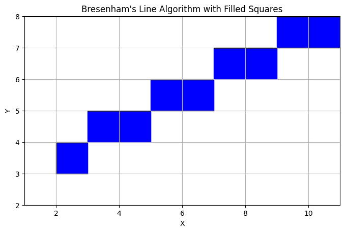
p5.js
function setup() {
  createCanvas(400, 400);
  background(0); // Set background to black
}

function draw() {
  // Draw line from (10, 10) to (300, 300)
  bresenhamLineAllOctants(10, 10, 300, 300);
  noLoop(); // Stops draw loop
}
function bresenhamLineAllOctants(x1, y1, x2, y2) {
  // Determine differences and step directions
  let deltaX = x2 - x1;
  let deltaY = y2 - y1;
  let stepX = deltaX >= 0 ? 1 : -1;
  let stepY = deltaY >= 0 ? 1 : -1;
  deltaX = Math.abs(deltaX);
  deltaY = Math.abs(deltaY);

  // Initialize starting points and decision variable
  let x = x1;
  let y = y1;
  let linePoints = [[x, y]]; // Store points of the line
  let nablaI;

  if (deltaX >= deltaY) {
    nablaI = 2 * deltaY - deltaX;
    while (x != x2) {
      x += stepX;
      if (nablaI > 0) {
        y += stepY;
        nablaI -= 2 * deltaX;
      }
      nablaI += 2 * deltaY;
      linePoints.push([x, y]);
    }
  } else {
    nablaI = 2 * deltaX - deltaY;
    while (y != y2) {
      y += stepY;
      if (nablaI > 0) {
        x += stepX;
        nablaI -= 2 * deltaY;
      }
      nablaI += 2 * deltaX;
      linePoints.push([x, y]);
    }
  }

  // Drawing the line points on the canvas
  stroke(255); // White color for the line
  for (let i = 0; i < linePoints.length; i++) {
    point(linePoints[i][0], linePoints[i][1]); // Correctly refer to each point
  }
}
この記事が気に入ったらサポートをしてみませんか?