
[Python]医療費データ160次元をクラスター分析してみた:階層的クラスタリング

はじめに
こんにちは、機械学習勉強中のあおじるです。
今回は、以前の記事で使った医療費データ(160次元)を使ってクラスター分析をしてみます。
言語はPython、環境はGoogle Colaboratoryを使用しました。
使用するデータ
データは、以前の記事で作成した、全国健康保険協会(協会けんぽ)の加入者基本情報、医療費基本情報から作成した、10年間×47都道府県ごとの医療費の160次元のデータ(性別、年齢階級別の診療種別ごとの「医療費の3要素」)df_yt_C10_sn を使います。
(10年×47都道府県)×(10指標×性別2区分×年齢階級8区分)
= 470行 × 160次元
の形のデータです。
$$
\def\arraystretch{1.5}
\begin{array}{c:c|c:c:c:c}
\textsf{y} & \textsf{t} & \textsf{KperP\_1\_1\_1} & \textsf{KperP\_1\_1\_2} & \cdots & \textsf{TperN\_4\_2\_8} \\ \hline
2010 & 1 & {} & {} & {} & {} \\
2010 & 2 & {} & {} & {} & {} \\
\vdots & \vdots & \vdots & \vdots & \ddots & \vdots \\
2019 & 47 & {} & {} & {} & {}
\end{array}
$$
y:年度
2010~2019 の10年度分t:都道府県
1:北海道、・・・、47:沖縄 の47都道府県C10_s_n:性別s、年齢階級n別の10指標
KperP_1_1_1、KperP_1_1_2、・・・、TperN_4_2_8 の160項目C10:診療種別ごとの「医療費の3要素」で、XperY_k(診療種別kのYperX、YperX = Y/X)の形の10指標:
KperP_1:1人当たり件数_入院
KperP_2:1人当たり件数_外来
KperP_3:1人当たり件数_歯科
NperK_1:1件当たり日数_入院
NperK_2:1件当たり日数_外来
NperK_3:1件当たり日数_歯科
TperN_1:1日当たり点数_入院
TperN_2:1日当たり点数_外来
TperN_3:1日当たり点数_歯科
TperN_4:1日当たり点数_調剤
s:性別
1:男性、2:女性n:年齢階級
1:0~9歳、2:10~19歳、・・・、7:60~69歳、8:70歳以上
# 2010-2019年度データ
import pandas as pd
df = pd.read_csv('./df_yt_C10_sn.csv')
print(df.shape) # (470, 162)

# 数値部分のみ取り出し
X = df.iloc[:,2:]
print(X.shape) # (470, 160)

# スケーリング
from sklearn import preprocessing
scaler = preprocessing.MinMaxScaler()
X = scaler.fit_transform(X)
print(X.shape) # (470, 160)
階層的クラスタリング
1.データをそのままクラスタリング
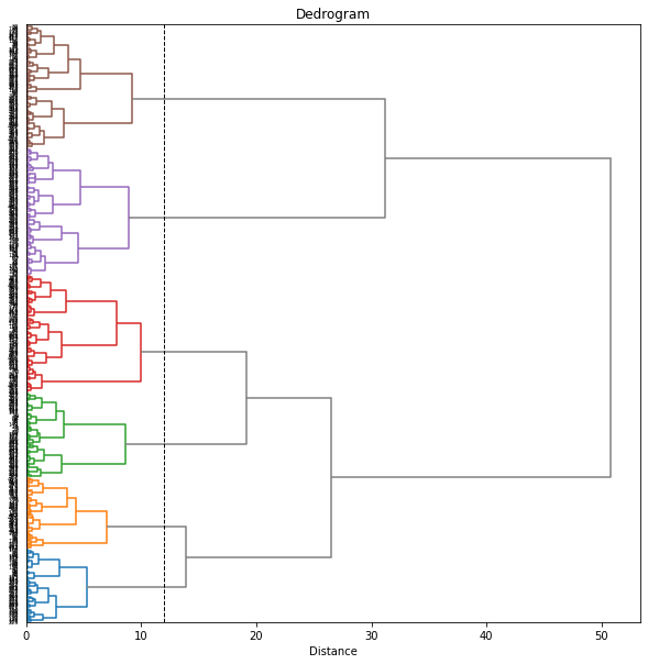
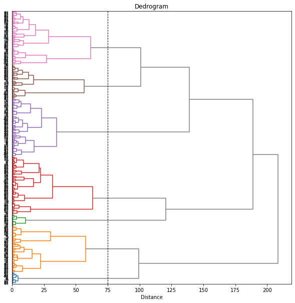
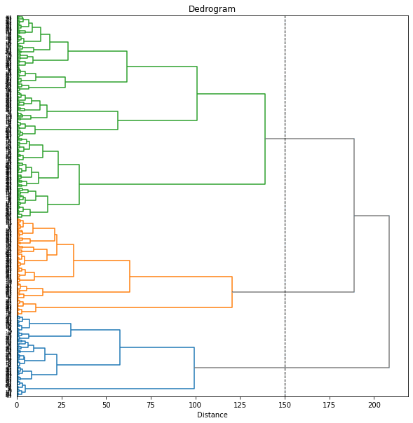
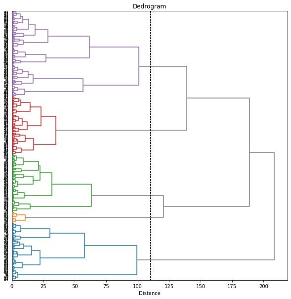
まず、160次元のデータをそのまま階層的クラスタリング(Hierarchical Clustering)します。
科学計算ライブラリの SciPy の scipy.cluster.hierarchy を用います。距離は通常のユークリッド距離(euclidean)、クラスタリングの手法はウォード法(ward)を用いました。
from scipy.cluster.hierarchy import linkage, fcluster, dendrogram

Z = linkage(X, method='ward', metric='euclidean')
# Z = ward(pdist(X, metric='euclidean'))

plt.figure(figsize=(10, 10))
dend = dendrogram(Z, orientation='right', labels=range(len(df)))
plt.title('Dedrogram')
plt.xlabel('Distance')
plt.yticks()
plt.show()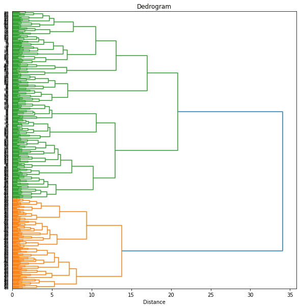
樹形図(dendrogram)をみて、閾値を12あたりにしてみると7個のクラスターに分けられました。
threshold = 12
print('Threshold: {}'.format(threshold))
clusters = fcluster(Z ,t=threshold, criterion='distance')
print('Clusters: \n{}'.format(clusters))
# print(set(clusters))
n_clusters = len(set(clusters))
print('Number of clusters: {}'.format(n_clusters))

plt.figure(figsize=(10, 10))
# plt.grid()
plt.axvline(x=threshold, ymin=0, ymax=1, c='k', linewidth=1, linestyle='dashed')
dend = dendrogram(Z, orientation='right', labels=range(len(df)),
                  color_threshold=threshold)
plt.title('Dedrogram')
plt.xlabel('Distance')
plt.yticks()
plt.show()

# Threshold: 12
# Clusters:
# [6 7 7 7 7 7 7 4 4 4 4 4 4 4 7 7 7 7 7 4 3 4 3 4 4 4 4 4 4 4 7 7 3 5 5 4 5
#  4 7 5 5 5 5 5 5 5 6 6 7 7 7 7 7 7 4 4 4 4 4 4 4 7 7 7 7 7 4 3 4 3 4 4 4 4
#  4 4 4 7 7 3 5 5 4 5 4 7 5 5 5 5 5 5 5 6 6 7 7 3 7 7 7 4 4 4 4 4 2 2 7 7 7
#  7 7 4 3 4 3 3 4 3 3 3 3 4 7 7 3 3 5 4 3 4 7 5 5 5 5 5 5 5 6 6 7 7 3 7 1 7
#  4 3 4 4 4 2 2 7 7 7 7 7 1 3 4 3 3 4 3 3 3 3 3 7 7 3 3 5 3 3 4 7 5 5 5 5 5
#  5 5 6 6 7 7 3 7 1 7 4 3 3 4 2 2 2 1 7 7 7 7 1 3 4 2 3 4 3 3 3 3 3 7 7 2 3
#  3 3 3 4 7 5 5 3 5 7 5 5 6 6 7 7 3 7 1 1 2 3 3 2 2 2 2 1 1 7 7 1 1 2 4 2 3
#  2 2 2 3 3 3 7 1 2 3 3 3 1 3 7 3 3 3 5 7 5 5 6 6 1 7 3 1 1 1 2 3 3 2 2 2 2
#  1 1 7 7 1 1 2 4 2 3 2 2 2 2 3 3 7 1 2 3 3 3 1 3 7 3 3 3 5 7 5 5 6 6 1 1 2
#  1 1 1 2 3 3 2 2 2 2 1 1 7 7 1 1 2 2 2 2 2 2 2 2 2 3 7 1 2 2 3 1 1 3 1 3 3
#  3 3 7 7 3 6 6 1 1 2 1 1 1 2 3 3 2 2 2 2 1 1 1 1 1 1 2 2 2 2 2 2 2 2 2 1 1
#  1 2 2 3 1 1 3 1 3 3 3 3 7 7 3 6 6 1 1 2 1 1 1 2 3 3 2 2 2 2 1 1 1 1 1 1 2
#  2 2 2 2 2 2 2 2 1 1 1 2 2 3 1 1 3 1 3 3 3 3 7 7 3 6]
# Number of clusters: 7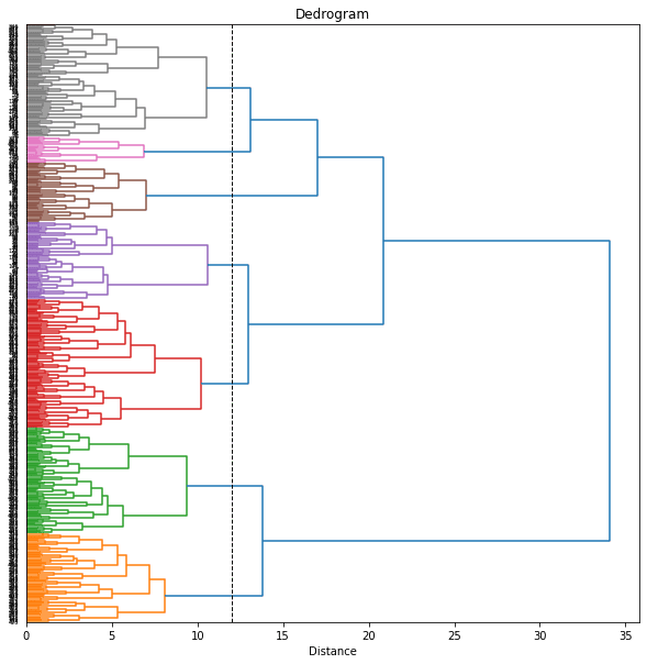
樹形図のクラスターは自動で色分けされますが、後でその色分けを使いたいので、seabornのカラーパレットを用いて、樹形図に使われる色をあらかじめ設定しておくことにします。
# カラーパレット
import seaborn as sns
cp = sns.color_palette(n_colors=n_clusters)
sns.palplot(cp)
print(cp)
# [(0.12156862745098039, 0.4666666666666667, 0.7058823529411765), ...]
from matplotlib.colors import rgb2hex
print([rgb2hex(rgb) for rgb in cp])
# ['#1f77b4', '#ff7f0e', '#2ca02c', '#d62728', '#9467bd', '#8c564b', '#e377c2']
樹形図を描く関数 dendrogram は辞書型の返り値を返しますが、その中の 'leaves_color_list' に樹形図上で(クラスターごとに)色分けされた各データの色が保存されています。(なお、dendrogram 関数の返す辞書型のうちの 'leaves_color_list' は、scipy 1.7.1 以降のバージョンで新しく使えるようになった機能のようです(参照)。現在(2022/06/26)、Google Colaboratory にインストールされているScipyのバージョンは 1.4.1 でしたので、アップグレードして使いました。)
print(dend['leaves_color_list'])
# KeyError: 'leaves_color_list'


import scipy as sp
# バージョン確認
print(sp.version.full_version)
# 1.4.1

# 最新バージョンにアップグレード
!pip install --upgrade scipy

# バージョン確認
import scipy as sp
print(sp.version.full_version)
# 1.7.3

# RESTART RUNTIME
# (バージョンアップ後はランタイムを再起動する必要あり。)

print(dend['leaves_color_list'])
# ['C1', 'C1', 'C1', 'C1', 'C1', ...]このカラーパレットで樹形図の色を設定します(set_link_color_palette)。
from scipy.cluster.hierarchy import set_link_color_palette

plt.figure(figsize=(10, 10))
plt.axvline(x=threshold, ymin=0, ymax=1, c='k', linewidth=1, linestyle='dashed')
set_link_color_palette([rgb2hex(rgb) for rgb in cp])
dend = dendrogram(Z, orientation='right', labels=range(len(df)),
                  color_threshold=threshold, above_threshold_color='gray')
set_link_color_palette(None)  # reset to default after use
plt.title('Dedrogram')
plt.xlabel('Distance')
plt.yticks()
plt.show()
cp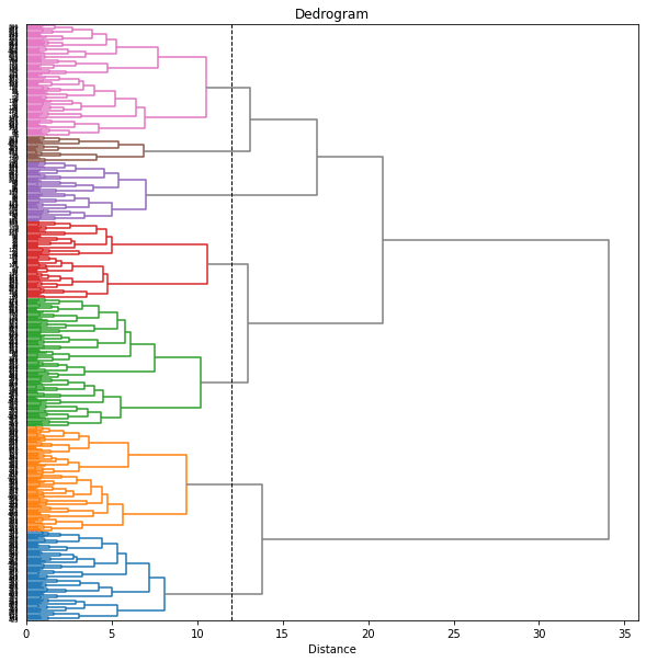
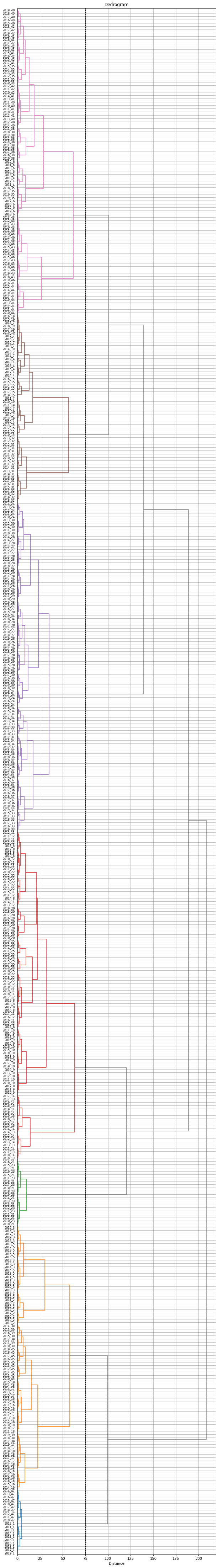
ラベルが見づらいので、もう少し大きくしてみます。樹形図上で、同じ都道府県の年度違いのデータはまとまって出てきているのがわかります。
labels = ['{}_{}'.format(df['y'][i], df['t'][i]) for i in range(len(df))]

plt.figure(figsize=(10, 80))
plt.axvline(x=threshold, ymin=0, ymax=1, c='k', linewidth=1, linestyle='dashed')
plt.grid()
set_link_color_palette([rgb2hex(rgb) for rgb in cp])
dend = dendrogram(Z, orientation='right', labels=labels,
                  color_threshold=threshold, above_threshold_color='gray')
set_link_color_palette(None)  # reset to default after use
plt.title('Dedrogram')
plt.xlabel('Distance')
plt.yticks(size=8)
plt.show()
cp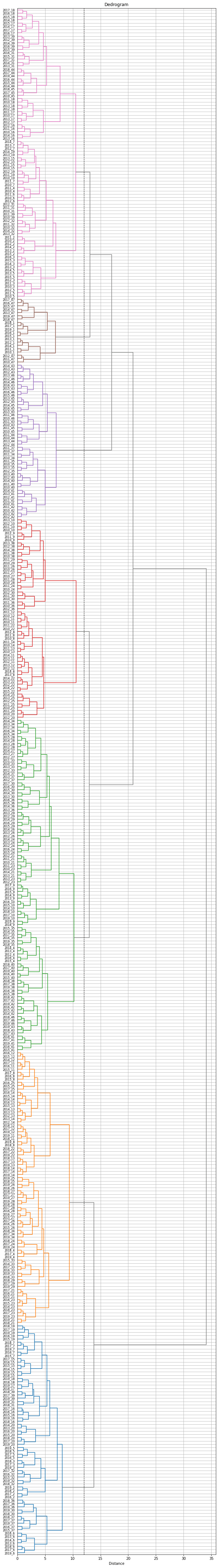
これで、各都道府県の10年分のデータ(47×10=470データ)が7つのクラスターに分けられました。
ただし、同じ都道府県でも年度によって異なるクラスターに属しているものがあります。そこで、都道府県ごとに10年分のデータのうち最も多くの年度が属するクラスターをその都道府県のクラスターとすることにします。
df_cluster = df.copy()
df_cluster['cluster'] = clusters
df_cluster['n'] = 1
df_cluster = df_cluster.loc[:,['t','cluster','n']] \
                       .groupby(['t', 'cluster'], as_index=False) \
                       .sum() \
                       .sort_values(['t', 'n'], ascending=[True, False]) \
                       .drop_duplicates(subset='t', keep='first') \
                       .reset_index() \
                       .loc[:,['t', 'cluster', 'n']]
print(df_cluster.shape)
# (47, 3)
print(df_cluster)
#      t  cluster   n
# 0    1        6  10
# 1    2        7   6
# 2    3        7   7
# 3    4        3   5
# 4    5        7   6
# 5    6        1   7
# 6    7        1   5
# 7    8        2   5
# 8    9        3   7
# 9   10        3   6
# 10  11        2   5
# 11  12        2   6
# 12  13        2   8
# 13  14        2   8
# 14  15        1   6
# 15  16        1   5
# 16  17        7   8
# 17  18        7   8
# 18  19        1   5
# 19  20        1   7
# 20  21        2   5
# 21  22        4   7
# 22  23        2   6
# 23  24        3   5
# 24  25        2   5
# 25  26        2   5
# 26  27        2   5
# 27  28        2   4
# 28  29        3   5
# 29  30        3   5
# 30  31        7   8
# 31  32        1   5
# 32  33        2   6
# 33  34        3   5
# 34  35        3   6
# 35  36        3   4
# 36  37        1   5
# 37  38        3   5
# 38  39        7   7
# 39  40        3   5
# 40  41        3   5
# 41  42        3   6
# 42  43        5   7
# 43  44        7   6
# 44  45        5   7
# 45  46        5   7
# 46  47        6  10
これで、47都道府県を7つのクラスターに分けることができました。(北海道と沖縄以外は年度によって異なるクラスターに属していました。最も多くの年度が属するクラスターに振り分けましたが、最も多くの年度が4年度しかない都道府県もあり、あまりうまく分けられているとは言えません。)
最後に、都道府県のクラスター分けの結果を日本地図上に色分けして表示しておきます。日本地図を県別に色分けするための japanmap というライブラリを使いました。
! pip install japanmapfrom japanmap import pref_names
dict_cluster = {pref_names[t]: df_cluster['cluster'][t-1] for t in range(1,47+1,1)}
print(dict_cluster)
# {'北海道': 6, '青森県': 7, '岩手県': 7, '宮城県': 3, '秋田県': 7, '山形県': 1, ...}
dict_color = {pref_names[t]: rgb2hex(cp[df_cluster['cluster'][t-1]-1]) \
for t in range(1,47+1,1)}
print(dict_color)
# {'北海道': '#8c564b', '青森県': '#e377c2', '岩手県': '#e377c2', ...}
from japanmap import picture
plt.figure(figsize=(8,8))
plt.imshow(picture(dict_color))
plt.tick_params(bottom=False, top=False, left=False, right=False,
labelbottom=False, labeltop=False, labelleft=False, labelright=False)
plt.show()
cp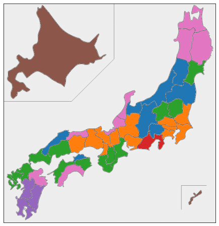
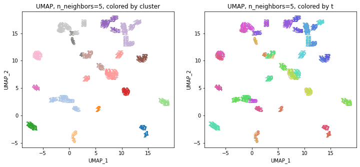
2.UMAPの結果をクラスタリング
160次元のデータをそのままクラスタリングするのはあまりうまくいきませんでしたので、UMAPで圧縮した2次元のデータを使ってクラスタリングしてみます。
以前の記事で、UMAPのパラメータとして n_neighbors = 30 がバランスがとれてよさそうでしたので、その結果を使います。
! pip install umap-learn

# UMAP
import umap.umap_ as umap

n_neighbors = 30
reducer = umap.UMAP(n_components=2, n_neighbors=n_neighbors, random_state=0)
reducer.fit(X)
embedding = reducer.transform(X)
print(embedding.shape) # (470, 2)

XX = embedding
print(XX.shape) # (470, 2)
1.と同じようにクラスタリングします。
from scipy.cluster.hierarchy import linkage, fcluster, dendrogram

Z = linkage(XX, method='ward', metric='euclidean')

plt.figure(figsize=(10, 10))
dend = dendrogram(Z, orientation='right', labels=range(len(df)))
plt.title('Dedrogram')
plt.xlabel('Distance')
plt.yticks()
plt.show()

threshold = 12
print('Threshold: {}'.format(threshold))
clusters = fcluster(Z ,t=threshold, criterion='distance')
print('Clusters: \n{}'.format(clusters))
# print(set(clusters))
n_clusters = len(set(clusters))
print('Number of clusters: {}'.format(n_clusters))

import seaborn as sns
cp = sns.color_palette(n_colors=n_clusters)
sns.palplot(cp)

from scipy.cluster.hierarchy import set_link_color_palette
plt.figure(figsize=(10, 10))
plt.axvline(x=threshold, ymin=0, ymax=1, c='k', linewidth=1, linestyle='dashed')
set_link_color_palette([rgb2hex(rgb) for rgb in cp])
dend = dendrogram(Z, orientation='right', labels=range(len(df)),
                  color_threshold=threshold, above_threshold_color='gray')
set_link_color_palette(None)  # reset to default after use
plt.title('Dedrogram')
plt.xlabel('Distance')
plt.yticks()
plt.show()
cp

# Threshold: 12
# Clusters:
# [4 3 3 3 3 2 3 5 5 5 5 5 5 5 3 4 4 4 3 5 6 5 6 6 5 6 6 6 6 6 4 4 6 2 1 2 2
#  1 4 1 1 1 1 1 1 1 4 4 3 3 2 3 2 3 5 5 5 5 5 5 5 3 4 4 4 3 5 6 5 6 6 5 6 6
#  6 6 6 4 4 6 2 1 2 2 1 4 1 1 1 1 1 1 1 4 4 3 3 2 3 2 3 5 5 5 5 5 5 5 3 4 4
#  4 3 5 6 5 6 6 5 6 6 6 6 6 4 4 6 2 1 2 2 1 4 1 1 1 1 1 1 1 4 4 3 3 2 3 2 3
#  5 5 5 5 5 5 5 3 4 4 4 3 5 6 5 6 6 5 6 6 6 6 6 4 4 6 6 1 2 2 1 4 1 1 1 1 1
#  1 1 4 4 3 3 3 3 2 3 5 5 5 5 5 5 5 3 4 4 4 3 5 6 5 6 6 5 6 6 6 6 6 4 4 6 6
#  1 2 2 1 4 1 1 1 1 4 4 1 4 4 3 3 3 3 2 3 5 5 5 5 5 5 5 3 4 4 4 3 5 6 5 6 6
#  5 6 6 6 6 6 4 4 6 6 2 2 2 1 4 1 1 1 1 4 4 1 4 4 3 3 3 3 2 3 5 5 5 5 5 5 5
#  3 4 4 4 3 5 6 5 6 6 5 6 6 6 6 6 4 4 6 6 2 2 2 2 4 1 1 1 1 4 4 1 4 4 3 3 3
#  3 2 3 5 5 5 5 5 5 5 3 4 4 4 3 5 6 5 6 6 5 6 6 6 6 6 4 4 6 6 2 2 2 2 4 2 1
#  2 1 4 4 1 4 4 3 3 3 3 2 3 5 5 5 5 5 5 5 3 4 4 4 3 5 6 5 6 6 5 6 6 6 6 6 4
#  4 6 6 2 2 2 2 4 2 2 2 2 4 4 1 4 4 3 3 3 3 2 3 5 5 5 5 5 5 5 3 4 4 4 3 5 6
#  5 6 6 5 6 6 6 6 6 4 4 6 6 2 2 2 2 4 2 2 2 2 4 4 2 4]
# Number of clusters: 6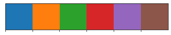
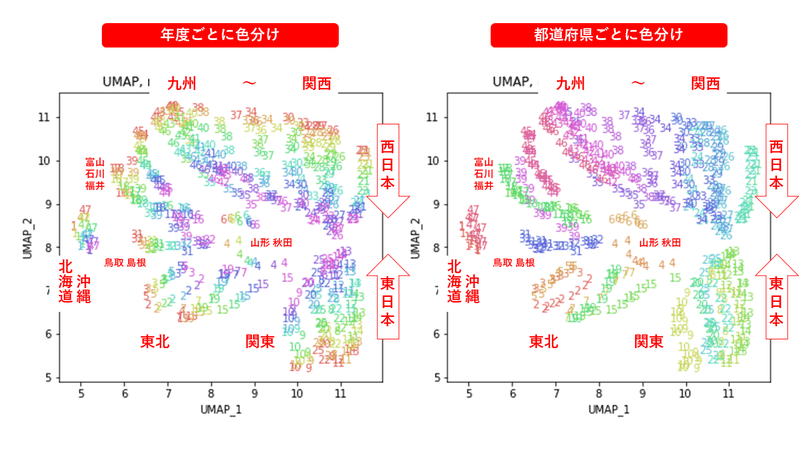
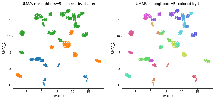
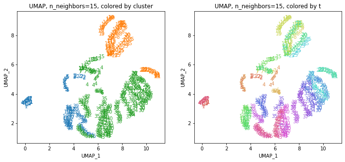
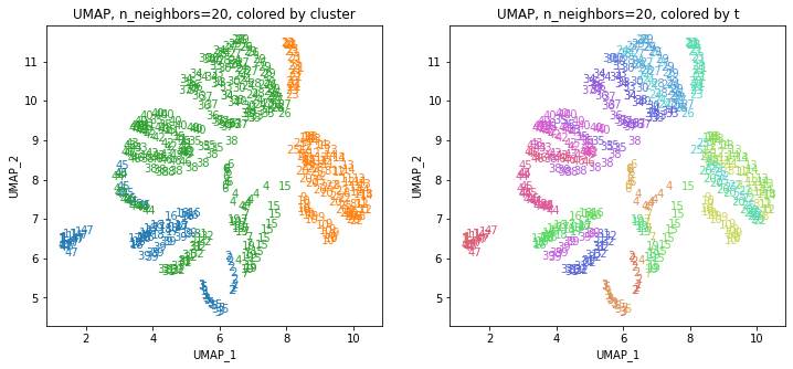
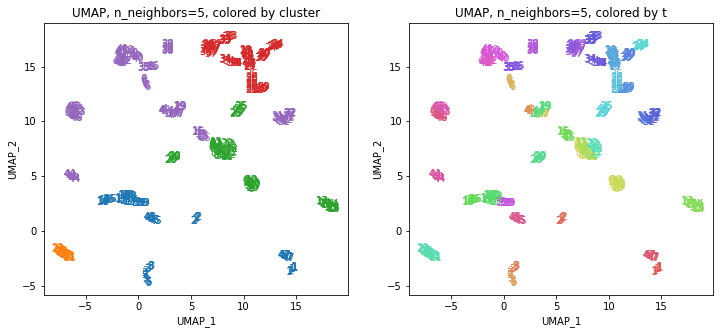
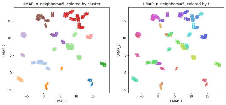
UMAPの結果の2次元上にクラスタリングの結果を色分けして表示してみます。
alg = 'UMAP' # algorithm
param = 'n_neighbors='+str(n_neighbors) # parameter

print('{}, {}'.format(alg,param))
xmin, xmax = min(XX[:,0]), max(XX[:,0])
ymin, ymax = min(XX[:,1]), max(XX[:,1])
plt.figure(figsize=(12,5))
plt.subplot(1, 2, 1)
plt.title('{}, {}, colored by cluster'.format(alg,param))
plt.xlabel('{}_{}'.format(alg,1))
plt.ylabel('{}_{}'.format(alg,2))
plt.xlim(xmin-(xmax-xmin)/20, xmax+(xmax-xmin)/20)
plt.ylim(ymin-(ymax-ymin)/20, ymax+(ymax-ymin)/20)
for p in range(10*47):
  plt.text(x=XX[dend['leaves'][p],0], y=XX[dend['leaves'][p],1],
           s=df.iloc[dend['leaves'][p],1], color=dend['leaves_color_list'][p],
           ha='center', va='center', fontsize=10)
plt.subplot(1, 2, 2)
plt.title('{}, {}, colored by t'.format(alg,param))
plt.xlabel('{}_{}'.format(alg,1))
plt.ylabel('{}_{}'.format(alg,2))
plt.xlim(xmin-(xmax-xmin)/20, xmax+(xmax-xmin)/20)
plt.ylim(ymin-(ymax-ymin)/20, ymax+(ymax-ymin)/20)
for p in range(10*47):
  plt.text(x=XX[p,0], y=XX[p,1], s=df.iloc[p,1], color=color_t[p],
           ha='center', va='center', fontsize=10)
plt.show()
cp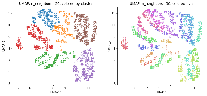
左の図がクラスタリングの結果で、6つのクラスターに色分けされています。右の図は、以前の記事と同じ都道府県別の色分けです。左右の図を見比べると、クラスタリングの結果は同じ都道府県は概ね同じクラスター(同じ色)に分かれていますが、年度によって別のクラスター(別の色)に分けられているところもあります(青とオレンジのところなど)。
1.と同様に、10年分のデータのうち最も多くの年度が属するクラスターでその都道府県のクラスターを決めます。
df_cluster = df.copy()
df_cluster['cluster'] = clusters
df_cluster['n'] = 1
df_cluster = df_cluster.loc[:,['t','cluster','n']] \
                       .groupby(['t', 'cluster'], as_index=False) \
                       .sum() \
                       .sort_values(['t', 'n'], ascending=[True, False]) \
                       .drop_duplicates(subset='t', keep='first') \
                       .reset_index() \
                       .loc[:,['t', 'cluster', 'n']]
print(df_cluster.shape)
# (47, 3)
print(df_cluster)
#      t  cluster   n
# 0    1        4  10
# 1    2        3  10
# 2    3        3  10
# 3    4        3   7
# 4    5        3  10
# 5    6        2  10
# 6    7        3  10
# 7    8        5  10
# 8    9        5  10
# 9   10        5  10
# 10  11        5  10
# 11  12        5  10
# 12  13        5  10
# 13  14        5  10
# 14  15        3  10
# 15  16        4  10
# 16  17        4  10
# 17  18        4  10
# 18  19        3  10
# 19  20        5  10
# 20  21        6  10
# 21  22        5  10
# 22  23        6  10
# 23  24        6  10
# 24  25        5  10
# 25  26        6  10
# 26  27        6  10
# 27  28        6  10
# 28  29        6  10
# 29  30        6  10
# 30  31        4  10
# 31  32        4  10
# 32  33        6  10
# 33  34        6   7
# 34  35        1   5
# 35  36        2  10
# 36  37        2  10
# 37  38        1   6
# 38  39        4  10
# 39  40        1   7
# 40  41        1   8
# 41  42        1   7
# 42  43        1   8
# 43  44        4   6
# 44  45        4   6
# 45  46        1   9
# 46  47        4  10

from japanmap import pref_names
dict_cluster = {pref_names[t]: df_cluster['cluster'][t-1] for t in range(1,47+1,1)}
print(dict_cluster)
dict_color = {pref_names[t]: rgb2hex(cp[df_cluster['cluster'][t-1]-1]) \
              for t in range(1,47+1,1)}
print(dict_color)

from japanmap import picture
plt.figure(figsize=(8,8))
plt.imshow(picture(dict_color))
plt.tick_params(bottom=False, top=False, left=False, right=False,
                labelbottom=False, labeltop=False, labelleft=False, labelright=False)
plt.show()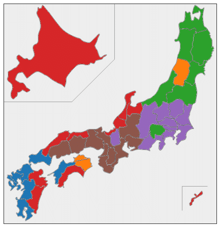
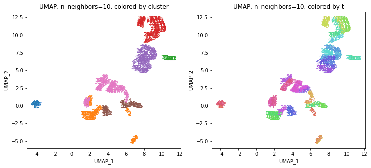
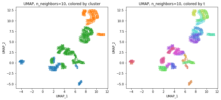
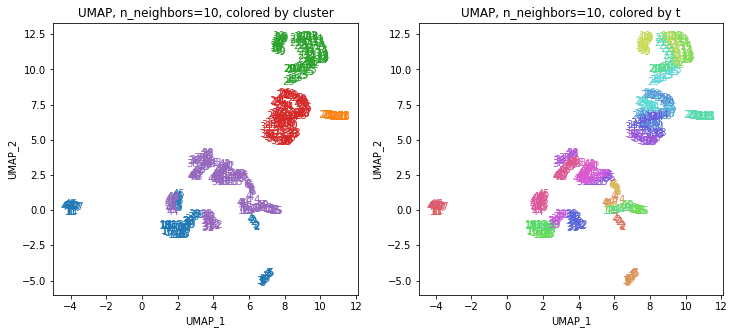
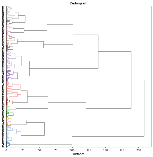
3.複数のUMAPの結果をまとめてクラスタリング
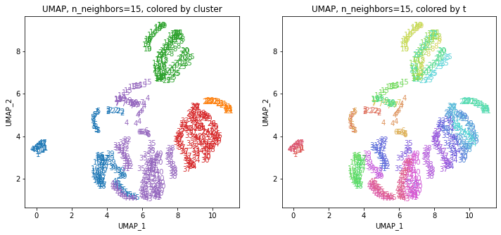
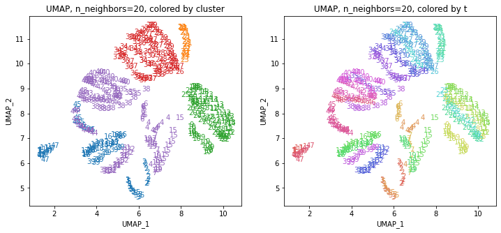
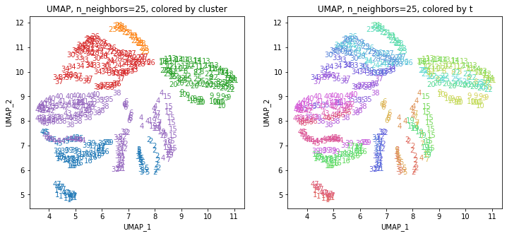
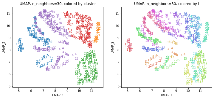
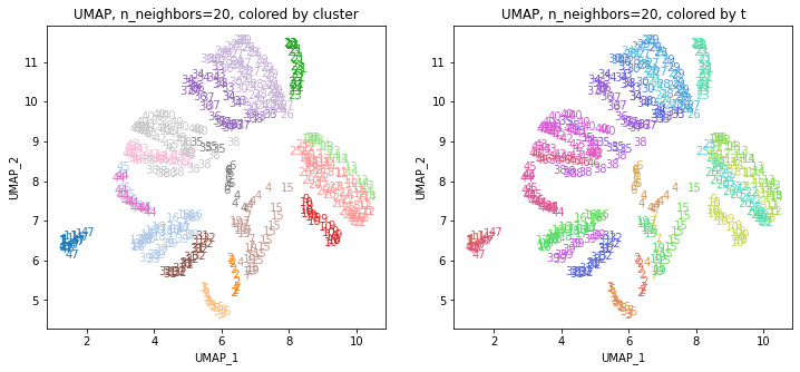
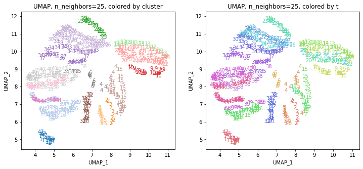
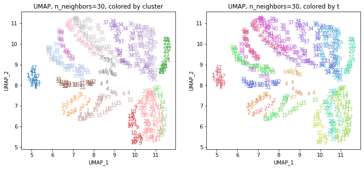
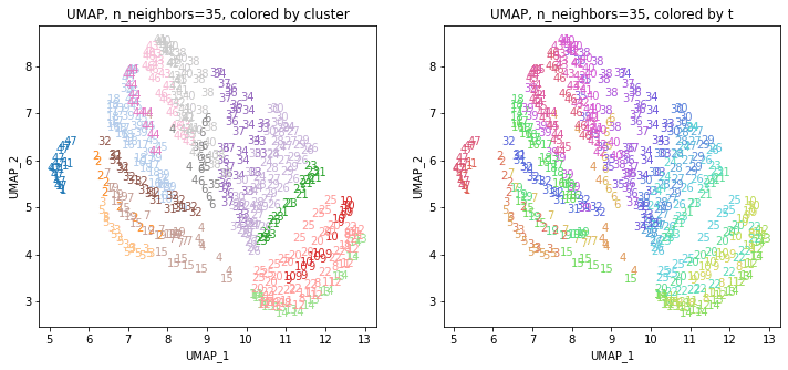
以前の記事で、UMAPのパラメータ n_neighbors を変化させると、都道府県ごとの結果がうまくまとまって動いていました。そこで、パラメータを変化させたときの複数のUMAPの結果をまとめたデータでクラスタリングしてみます。パラメータ n_neighbors を5~50まで変化させてそれらの結果を使います。
list_n_neighbors = [5,10,15,20,25,30,35,40,50]

k = len(list_n_neighbors)

import numpy as np
XX = np.zeros((470, 2*k))
print(XX.shape) # (470, 18)
for i in range(k):
  n_neighbors = list_n_neighbors[i]
  print(n_neighbors)
  reducer = umap.UMAP(n_components=2, n_neighbors=n_neighbors, random_state=0)
  reducer.fit(X)
  embedding = reducer.transform(X)
  print(embedding.shape) # (470, 2)
  XX[:,i*2:i*2+2] = embedding
print(XX.shape) # (470, 18)
from scipy.cluster.hierarchy import linkage, fcluster, dendrogram
Z = linkage(XX, method='ward', metric='euclidean')
plt.figure(figsize=(10, 10))
dend = dendrogram(Z, orientation='right', labels=range(len(df)))
plt.title('Dedrogram')
plt.xlabel('Distance')
plt.yticks()
plt.show()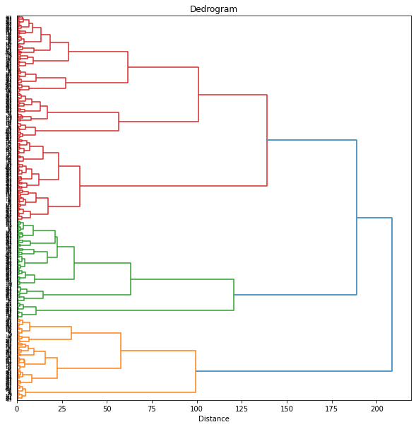
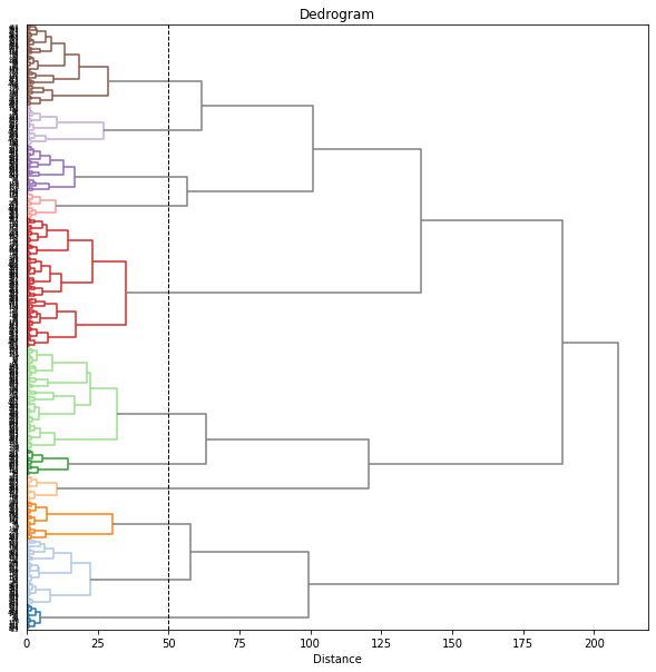
threshold = 75
threshold = 75
print('Threshold: {}'.format(threshold))
clusters = fcluster(Z ,t=threshold, criterion='distance')
print('Clusters: \n{}'.format(clusters))
# print(set(clusters))
n_clusters = len(set(clusters))
print('Number of clusters: {}'.format(n_clusters))
# Threshold: 75
# Clusters:
# [1 2 2 6 2 7 6 4 4 4 4 4 4 4 6 2 2 2 6 4 3 4 3 5 4 5 5 5 5 5 6 6 5 5 7 5 5
#  7 2 7 7 7 7 7 2 7 1 1 2 2 7 2 7 6 4 4 4 4 4 4 4 6 2 2 2 6 4 3 4 3 5 4 5 5
#  5 5 5 6 6 5 5 7 5 5 7 2 7 7 7 7 7 2 7 1 1 2 2 7 2 7 6 4 4 4 4 4 4 4 6 2 2
#  2 6 4 3 4 3 5 4 5 5 5 5 5 6 6 5 5 7 5 5 7 2 7 7 7 7 7 2 7 1 1 2 2 7 2 7 6
#  4 4 4 4 4 4 4 6 2 2 2 6 4 3 4 3 5 4 5 5 5 5 5 6 6 5 5 7 5 5 7 2 7 7 7 7 7
#  2 7 1 1 2 2 6 2 7 6 4 4 4 4 4 4 4 6 2 2 2 6 4 3 4 3 5 4 5 5 5 5 5 6 6 5 5
#  7 5 5 7 2 7 7 7 7 7 2 7 1 1 2 2 6 2 7 6 4 4 4 4 4 4 4 6 2 2 2 6 4 3 4 3 5
#  4 5 5 5 5 5 6 6 5 5 7 5 5 7 2 7 7 7 7 7 2 7 1 1 2 2 6 2 7 6 4 4 4 4 4 4 4
#  6 2 2 2 6 4 3 4 3 5 4 5 5 5 5 5 6 6 5 5 7 5 5 7 2 7 7 7 7 7 2 7 1 1 2 2 6
#  2 7 6 4 4 4 4 4 4 4 6 2 2 2 6 4 3 4 3 5 4 5 5 5 5 5 6 6 5 5 7 5 5 7 2 7 7
#  7 7 7 2 7 1 1 2 2 6 2 7 6 4 4 4 4 4 4 4 6 2 2 2 6 4 3 4 3 5 4 5 5 5 5 5 6
#  6 5 5 7 5 5 7 2 7 7 7 7 7 2 7 1 1 2 2 6 2 7 6 4 4 4 4 4 4 4 6 2 2 2 6 4 3
#  4 3 5 4 5 5 5 5 5 6 6 5 5 7 5 5 7 2 7 7 7 7 7 2 7 1]
# Number of clusters: 7

import seaborn as sns
if n_clusters <= 10:
  cp = sns.color_palette(n_colors=n_clusters)
elif n_clusters <= 20:
  cp = sns.color_palette('tab20', n_colors=n_clusters)
else:
  cp = sns.color_palette('Spectral', n_colors=n_clusters)
sns.palplot(cp)

from scipy.cluster.hierarchy import set_link_color_palette
plt.figure(figsize=(10, 10))
plt.axvline(x=threshold, ymin=0, ymax=1, c='k', linewidth=1, linestyle='dashed')
set_link_color_palette([rgb2hex(rgb) for rgb in cp])
dend = dendrogram(Z, orientation='right', labels=range(len(df)),
                  color_threshold=threshold, above_threshold_color='gray')
set_link_color_palette(None)  # reset to default after use
plt.title('Dedrogram')
plt.xlabel('Distance')
plt.yticks()
plt.show()

plt.figure(figsize=(10, 80))
plt.axvline(x=threshold, ymin=0, ymax=1, c='k', linewidth=1, linestyle='dashed')
plt.grid()
set_link_color_palette([rgb2hex(rgb) for rgb in cp])
dend = dendrogram(Z, orientation='right', labels=labels,
                  color_threshold=threshold, above_threshold_color='gray')
set_link_color_palette(None)  # reset to default after use
plt.title('Dedrogram')
plt.xlabel('Distance')
plt.yticks(size=8)
plt.show()
cp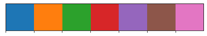
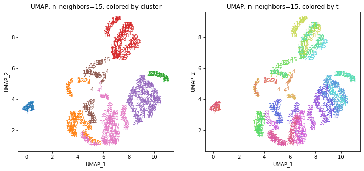
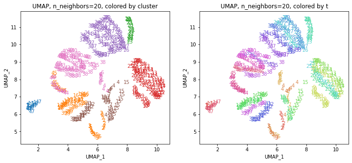
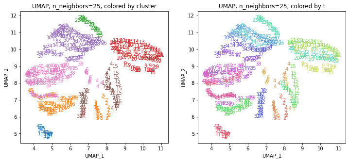
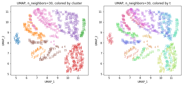
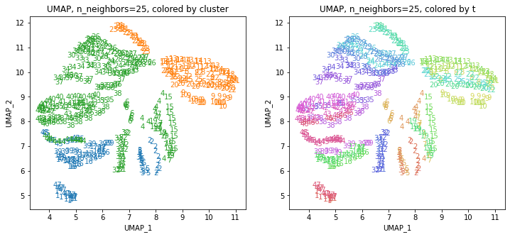
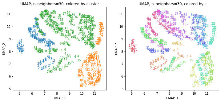
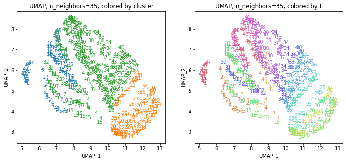
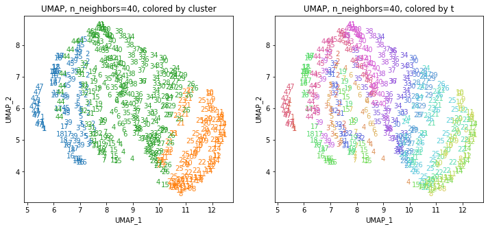
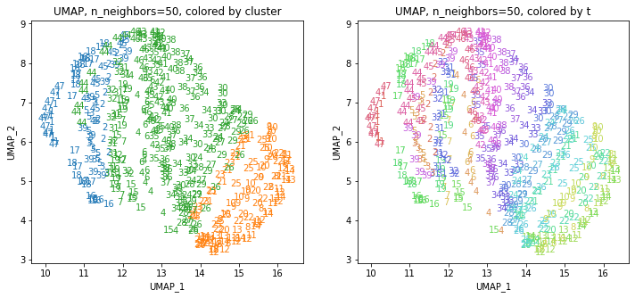
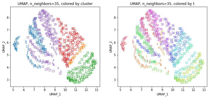
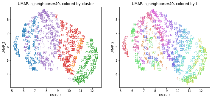
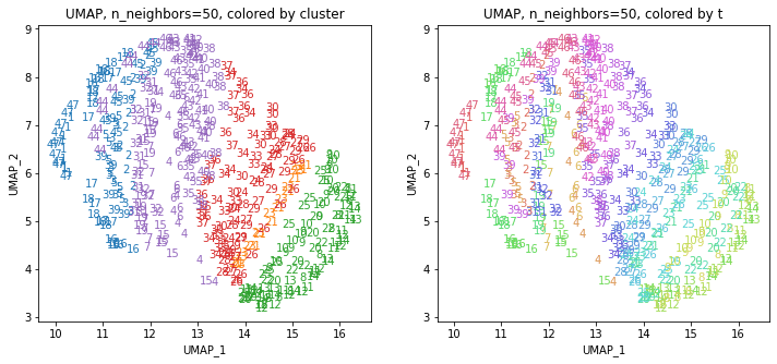
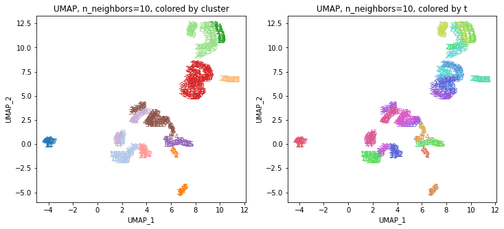
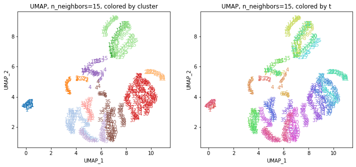
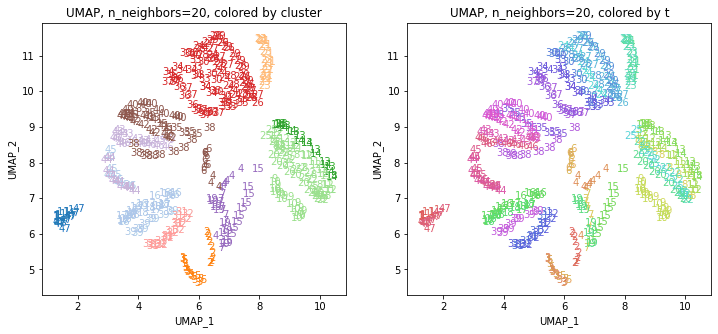
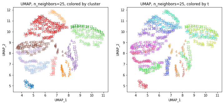
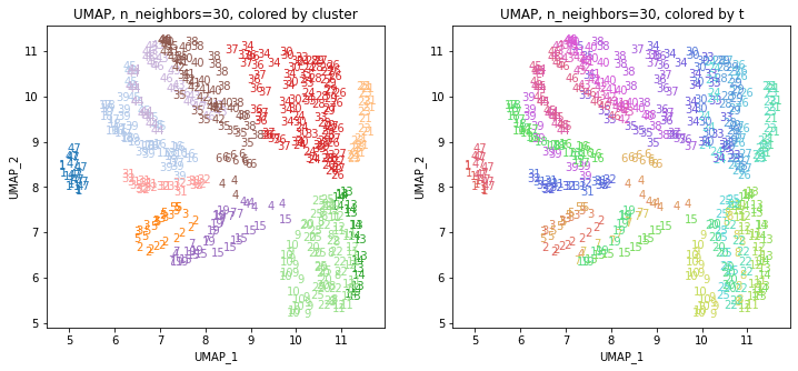
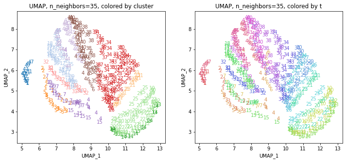
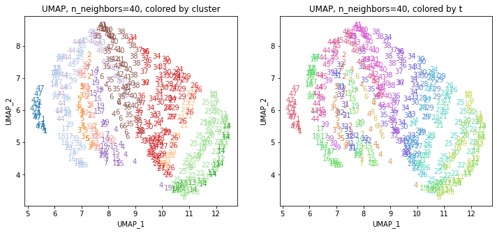
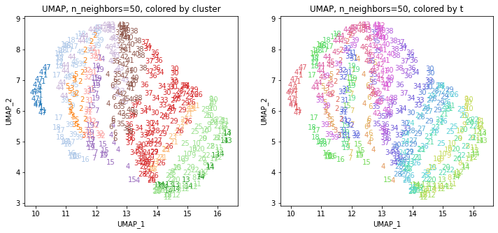
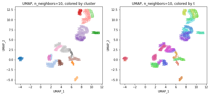
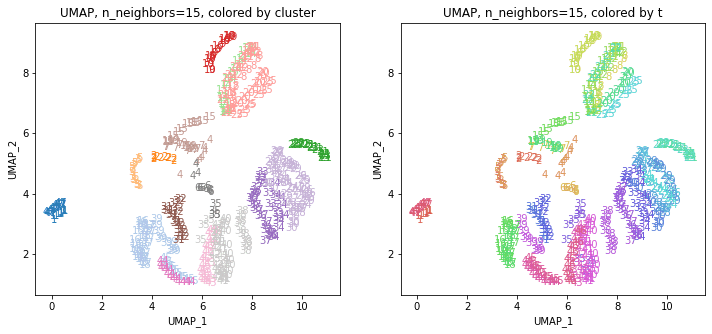
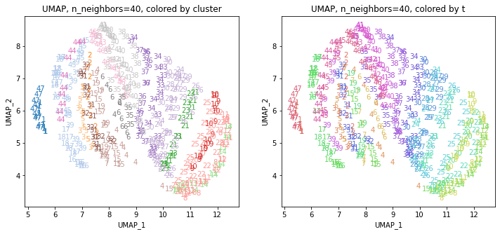
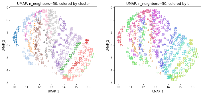
UMAPの結果の2次元上にクラスタリングの結果を色分けして表示してみます。
for i in range(k):
  n_neighbors = list_n_neighbors[i]
  print(n_neighbors)

  param = 'n_neighbors='+str(n_neighbors)

  print('{}, {}'.format(alg,param))
  xmin, xmax = min(XX[:,i*2]), max(XX[:,i*2])
  ymin, ymax = min(XX[:,i*2+1]), max(XX[:,i*2+1])
  plt.figure(figsize=(12,5))
  plt.subplot(1, 2, 1)
  plt.title('{}, {}, colored by cluster'.format(alg,param))
  plt.xlabel('{}_{}'.format(alg,1))
  plt.ylabel('{}_{}'.format(alg,2))
  plt.xlim(xmin-(xmax-xmin)/20, xmax+(xmax-xmin)/20)
  plt.ylim(ymin-(ymax-ymin)/20, ymax+(ymax-ymin)/20)
  for p in range(10*47):
    plt.text(x=XX[dend['leaves'][p],i*2], y=XX[dend['leaves'][p],i*2+1],
             s=df.iloc[dend['leaves'][p],1], color=dend['leaves_color_list'][p],
             ha='center', va='center', fontsize=10)
  plt.subplot(1, 2, 2)
  plt.title('{}, {}, colored by t'.format(alg,param))
  plt.xlabel('{}_{}'.format(alg,1))
  plt.ylabel('{}_{}'.format(alg,2))
  plt.xlim(xmin-(xmax-xmin)/20, xmax+(xmax-xmin)/20)
  plt.ylim(ymin-(ymax-ymin)/20, ymax+(ymax-ymin)/20)
  for p in range(10*47):
    plt.text(x=XX[p,i*2], y=XX[p,i*2+1], s=df.iloc[p,1], color=color_t[p],
             ha='center', va='center', fontsize=10)
  plt.show()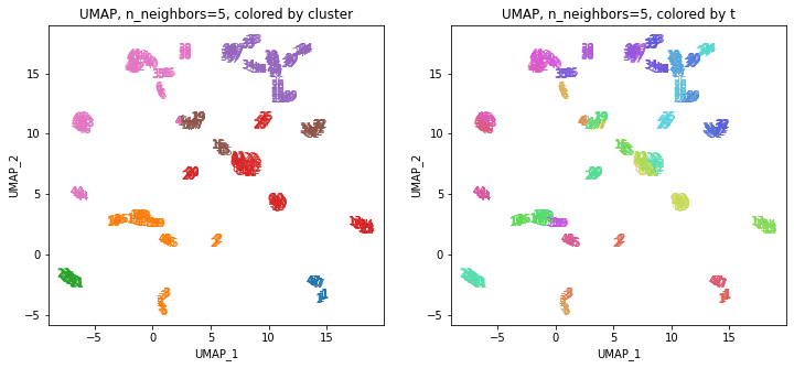
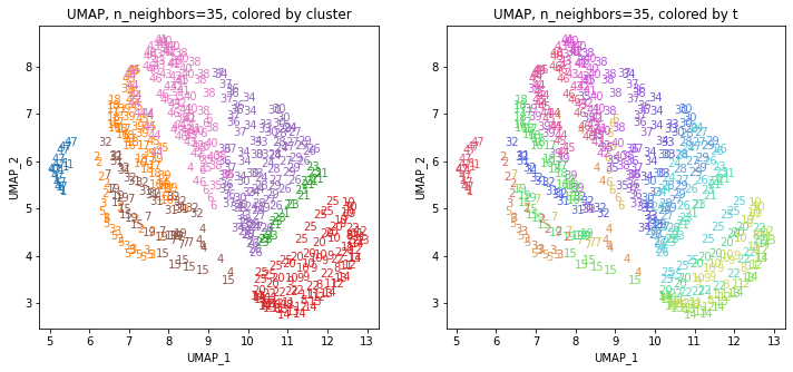
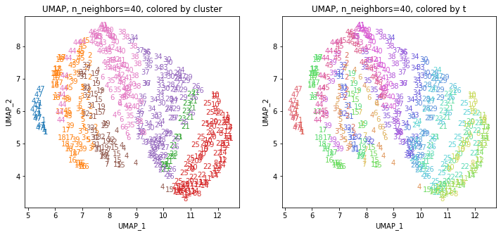
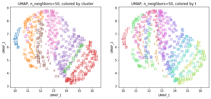
都道府県のクラスターを決めます。
df_cluster = df.copy()
df_cluster['cluster'] = clusters
df_cluster['n'] = 1
df_cluster = df_cluster.loc[:,['t','cluster','n']] \
.groupby(['t', 'cluster'], as_index=False) \
.sum() \
.sort_values(['t', 'n'], ascending=[True, False]) \
.drop_duplicates(subset='t', keep='first') \
.reset_index() \
.loc[:,['t', 'cluster', 'n']]
print(df_cluster.shape)
# (47, 3)
print(df_cluster)
# t cluster n
# 0 1 1 10
# 1 2 2 10
# 2 3 2 10
# 3 4 6 7
# 4 5 2 10
# 5 6 7 10
# 6 7 6 10
# 7 8 4 10
# 8 9 4 10
# 9 10 4 10
# 10 11 4 10
# 11 12 4 10
# 12 13 4 10
# 13 14 4 10
# 14 15 6 10
# 15 16 2 10
# 16 17 2 10
# 17 18 2 10
# 18 19 6 10
# 19 20 4 10
# 20 21 3 10
# 21 22 4 10
# 22 23 3 10
# 23 24 5 10
# 24 25 4 10
# 25 26 5 10
# 26 27 5 10
# 27 28 5 10
# 28 29 5 10
# 29 30 5 10
# 30 31 6 10
# 31 32 6 10
# 32 33 5 10
# 33 34 5 10
# 34 35 7 10
# 35 36 5 10
# 36 37 5 10
# 37 38 7 10
# 38 39 2 10
# 39 40 7 10
# 40 41 7 10
# 41 42 7 10
# 42 43 7 10
# 43 44 7 10
# 44 45 2 10
# 45 46 7 10
# 46 47 1 10
from japanmap import pref_names
dict_cluster = {pref_names[t]: df_cluster['cluster'][t-1] for t in range(1,47+1,1)}
print(dict_cluster)
dict_color = {pref_names[t]: rgb2hex(cp[df_cluster['cluster'][t-1]-1]) \
for t in range(1,47+1,1)}
print(dict_color)
from japanmap import picture
plt.figure(figsize=(8,8))
plt.imshow(picture(dict_color))
plt.tick_params(bottom=False, top=False, left=False, right=False,
labelbottom=False, labeltop=False, labelleft=False, labelright=False)
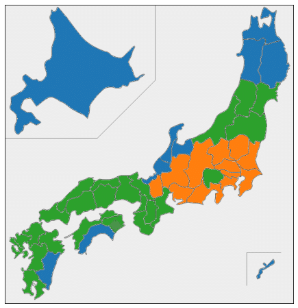
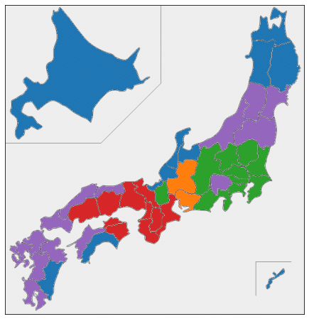
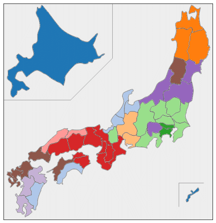
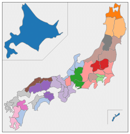
plt.show()ほぼすべての都道府県が10年分とも同じクラスターに分かれるという、ものすごくきれいな結果になりました。
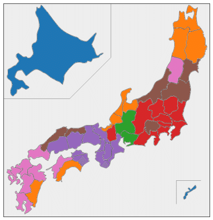
日本地図上の色分けをみると、地理的・文化的に近い都道府県が同じクラスターにうまく分かれている気がします。
閾値を変えた結果も示します。
threshold = 150
# Threshold: 150
# Clusters:
# [1 1 1 3 1 3 3 2 2 2 2 2 2 2 3 1 1 1 3 2 2 2 2 3 2 3 3 3 3 3 3 3 3 3 3 3 3
#  3 1 3 3 3 3 3 1 3 1 1 1 1 3 1 3 3 2 2 2 2 2 2 2 3 1 1 1 3 2 2 2 2 3 2 3 3
#  3 3 3 3 3 3 3 3 3 3 3 1 3 3 3 3 3 1 3 1 1 1 1 3 1 3 3 2 2 2 2 2 2 2 3 1 1
#  1 3 2 2 2 2 3 2 3 3 3 3 3 3 3 3 3 3 3 3 3 1 3 3 3 3 3 1 3 1 1 1 1 3 1 3 3
#  2 2 2 2 2 2 2 3 1 1 1 3 2 2 2 2 3 2 3 3 3 3 3 3 3 3 3 3 3 3 3 1 3 3 3 3 3
#  1 3 1 1 1 1 3 1 3 3 2 2 2 2 2 2 2 3 1 1 1 3 2 2 2 2 3 2 3 3 3 3 3 3 3 3 3
#  3 3 3 3 1 3 3 3 3 3 1 3 1 1 1 1 3 1 3 3 2 2 2 2 2 2 2 3 1 1 1 3 2 2 2 2 3
#  2 3 3 3 3 3 3 3 3 3 3 3 3 3 1 3 3 3 3 3 1 3 1 1 1 1 3 1 3 3 2 2 2 2 2 2 2
#  3 1 1 1 3 2 2 2 2 3 2 3 3 3 3 3 3 3 3 3 3 3 3 3 1 3 3 3 3 3 1 3 1 1 1 1 3
#  1 3 3 2 2 2 2 2 2 2 3 1 1 1 3 2 2 2 2 3 2 3 3 3 3 3 3 3 3 3 3 3 3 3 1 3 3
#  3 3 3 1 3 1 1 1 1 3 1 3 3 2 2 2 2 2 2 2 3 1 1 1 3 2 2 2 2 3 2 3 3 3 3 3 3
#  3 3 3 3 3 3 3 1 3 3 3 3 3 1 3 1 1 1 1 3 1 3 3 2 2 2 2 2 2 2 3 1 1 1 3 2 2
#  2 2 3 2 3 3 3 3 3 3 3 3 3 3 3 3 3 1 3 3 3 3 3 1 3 1]
# Number of clusters: 3

#      t  cluster   n
# 0    1        1  10
# 1    2        1  10
# 2    3        1  10
# 3    4        3  10
# 4    5        1  10
# 5    6        3  10
# 6    7        3  10
# 7    8        2  10
# 8    9        2  10
# 9   10        2  10
# 10  11        2  10
# 11  12        2  10
# 12  13        2  10
# 13  14        2  10
# 14  15        3  10
# 15  16        1  10
# 16  17        1  10
# 17  18        1  10
# 18  19        3  10
# 19  20        2  10
# 20  21        2  10
# 21  22        2  10
# 22  23        2  10
# 23  24        3  10
# 24  25        2  10
# 25  26        3  10
# 26  27        3  10
# 27  28        3  10
# 28  29        3  10
# 29  30        3  10
# 30  31        3  10
# 31  32        3  10
# 32  33        3  10
# 33  34        3  10
# 34  35        3  10
# 35  36        3  10
# 36  37        3  10
# 37  38        3  10
# 38  39        1  10
# 39  40        3  10
# 40  41        3  10
# 41  42        3  10
# 42  43        3  10
# 43  44        3  10
# 44  45        1  10
# 45  46        3  10
# 46  47        1  10
threshold = 110
# Threshold: 110
# Clusters:
# [1 1 1 5 1 5 5 3 3 3 3 3 3 3 5 1 1 1 5 3 2 3 2 4 3 4 4 4 4 4 5 5 4 4 5 4 4
#  5 1 5 5 5 5 5 1 5 1 1 1 1 5 1 5 5 3 3 3 3 3 3 3 5 1 1 1 5 3 2 3 2 4 3 4 4
#  4 4 4 5 5 4 4 5 4 4 5 1 5 5 5 5 5 1 5 1 1 1 1 5 1 5 5 3 3 3 3 3 3 3 5 1 1
#  1 5 3 2 3 2 4 3 4 4 4 4 4 5 5 4 4 5 4 4 5 1 5 5 5 5 5 1 5 1 1 1 1 5 1 5 5
#  3 3 3 3 3 3 3 5 1 1 1 5 3 2 3 2 4 3 4 4 4 4 4 5 5 4 4 5 4 4 5 1 5 5 5 5 5
#  1 5 1 1 1 1 5 1 5 5 3 3 3 3 3 3 3 5 1 1 1 5 3 2 3 2 4 3 4 4 4 4 4 5 5 4 4
#  5 4 4 5 1 5 5 5 5 5 1 5 1 1 1 1 5 1 5 5 3 3 3 3 3 3 3 5 1 1 1 5 3 2 3 2 4
#  3 4 4 4 4 4 5 5 4 4 5 4 4 5 1 5 5 5 5 5 1 5 1 1 1 1 5 1 5 5 3 3 3 3 3 3 3
#  5 1 1 1 5 3 2 3 2 4 3 4 4 4 4 4 5 5 4 4 5 4 4 5 1 5 5 5 5 5 1 5 1 1 1 1 5
#  1 5 5 3 3 3 3 3 3 3 5 1 1 1 5 3 2 3 2 4 3 4 4 4 4 4 5 5 4 4 5 4 4 5 1 5 5
#  5 5 5 1 5 1 1 1 1 5 1 5 5 3 3 3 3 3 3 3 5 1 1 1 5 3 2 3 2 4 3 4 4 4 4 4 5
#  5 4 4 5 4 4 5 1 5 5 5 5 5 1 5 1 1 1 1 5 1 5 5 3 3 3 3 3 3 3 5 1 1 1 5 3 2
#  3 2 4 3 4 4 4 4 4 5 5 4 4 5 4 4 5 1 5 5 5 5 5 1 5 1]
# Number of clusters: 5

#      t  cluster   n
# 0    1        1  10
# 1    2        1  10
# 2    3        1  10
# 3    4        5  10
# 4    5        1  10
# 5    6        5  10
# 6    7        5  10
# 7    8        3  10
# 8    9        3  10
# 9   10        3  10
# 10  11        3  10
# 11  12        3  10
# 12  13        3  10
# 13  14        3  10
# 14  15        5  10
# 15  16        1  10
# 16  17        1  10
# 17  18        1  10
# 18  19        5  10
# 19  20        3  10
# 20  21        2  10
# 21  22        3  10
# 22  23        2  10
# 23  24        4  10
# 24  25        3  10
# 25  26        4  10
# 26  27        4  10
# 27  28        4  10
# 28  29        4  10
# 29  30        4  10
# 30  31        5  10
# 31  32        5  10
# 32  33        4  10
# 33  34        4  10
# 34  35        5  10
# 35  36        4  10
# 36  37        4  10
# 37  38        5  10
# 38  39        1  10
# 39  40        5  10
# 40  41        5  10
# 41  42        5  10
# 42  43        5  10
# 43  44        5  10
# 44  45        1  10
# 45  46        5  10
# 46  47        1  10
threshold = 50
# Threshold: 50
# Clusters:
# [ 1  3  3  9  3 11  9  6  6  6  6  6  5  5  9  2  2  2  9  6  4  6  4  7
#   6  7  7  7  7  7  8  8  7  7 11  7  7 11  2 11 11 11 10 10  2 10  1  1
#   3  3 11  3 11  9  6  6  6  6  6  5  5  9  2  2  2  9  6  4  6  4  7  6
#   7  7  7  7  7  8  8  7  7 11  7  7 11  2 11 11 11 10 10  2 10  1  1  3
#   3 11  3 11  9  6  6  6  6  6  5  5  9  2  2  2  9  6  4  6  4  7  6  7
#   7  7  7  7  8  8  7  7 11  7  7 11  2 11 11 11 10 10  2 10  1  1  3  3
#  11  3 11  9  6  6  6  6  6  5  5  9  2  2  2  9  6  4  6  4  7  6  7  7
#   7  7  7  8  8  7  7 11  7  7 11  2 11 11 11 10 10  2 10  1  1  3  3  9
#   3 11  9  6  6  6  6  6  5  5  9  2  2  2  9  6  4  6  4  7  6  7  7  7
#   7  7  8  8  7  7 11  7  7 11  2 11 11 11 10 10  2 10  1  1  3  3  9  3
#  11  9  6  6  6  6  6  5  5  9  2  2  2  9  6  4  6  4  7  6  7  7  7  7
#   7  8  8  7  7 11  7  7 11  2 11 11 11 10 10  2 10  1  1  3  3  9  3 11
#   9  6  6  6  6  6  5  5  9  2  2  2  9  6  4  6  4  7  6  7  7  7  7  7
#   8  8  7  7 11  7  7 11  2 11 11 11 10 10  2 10  1  1  3  3  9  3 11  9
#   6  6  6  6  6  5  5  9  2  2  2  9  6  4  6  4  7  6  7  7  7  7  7  8
#   8  7  7 11  7  7 11  2 11 11 11 10 10  2 10  1  1  3  3  9  3 11  9  6
#   6  6  6  6  5  5  9  2  2  2  9  6  4  6  4  7  6  7  7  7  7  7  8  8
#   7  7 11  7  7 11  2 11 11 11 10 10  2 10  1  1  3  3  9  3 11  9  6  6
#   6  6  6  5  5  9  2  2  2  9  6  4  6  4  7  6  7  7  7  7  7  8  8  7
#   7 11  7  7 11  2 11 11 11 10 10  2 10  1]
# Number of clusters: 11

#      t  cluster   n
# 0    1        1  10
# 1    2        3  10
# 2    3        3  10
# 3    4        9   7
# 4    5        3  10
# 5    6       11  10
# 6    7        9  10
# 7    8        6  10
# 8    9        6  10
# 9   10        6  10
# 10  11        6  10
# 11  12        6  10
# 12  13        5  10
# 13  14        5  10
# 14  15        9  10
# 15  16        2  10
# 16  17        2  10
# 17  18        2  10
# 18  19        9  10
# 19  20        6  10
# 20  21        4  10
# 21  22        6  10
# 22  23        4  10
# 23  24        7  10
# 24  25        6  10
# 25  26        7  10
# 26  27        7  10
# 27  28        7  10
# 28  29        7  10
# 29  30        7  10
# 30  31        8  10
# 31  32        8  10
# 32  33        7  10
# 33  34        7  10
# 34  35       11  10
# 35  36        7  10
# 36  37        7  10
# 37  38       11  10
# 38  39        2  10
# 39  40       11  10
# 40  41       11  10
# 41  42       11  10
# 42  43       10  10
# 43  44       10  10
# 44  45        2  10
# 45  46       10  10
# 46  47        1  10
threshold = 25
# Threshold: 25
# Clusters:
# [ 1  3  4 12  4 15 12  8  7  7  8  8  6  6 12  2  2  2 12  8  5  8  5 10
#   8 10 10 10 10 10 11 11  9  9 16  9  9 16  2 16 16 16 14 13  2 14  1  1
#   3  4 15  4 15 12  8  7  7  8  8  6  6 12  2  2  2 12  8  5  8  5 10  8
#  10 10 10 10 10 11 11  9  9 16  9  9 16  2 16 16 16 14 13  2 14  1  1  3
#   4 15  4 15 12  8  7  7  8  8  6  6 12  2  2  2 12  8  5  8  5 10  8 10
#  10 10 10 10 11 11  9  9 16  9  9 16  2 16 16 16 14 13  2 14  1  1  3  4
#  15  4 15 12  8  7  7  8  8  6  6 12  2  2  2 12  8  5  8  5 10  8 10 10
#  10 10 10 11 11  9  9 16  9  9 16  2 16 16 16 14 13  2 14  1  1  3  4 12
#   4 15 12  8  7  7  8  8  6  6 12  2  2  2 12  8  5  8  5 10  8 10 10 10
#  10 10 11 11  9  9 16  9  9 16  2 16 16 16 14 13  2 14  1  1  3  4 12  4
#  15 12  8  7  7  8  8  6  6 12  2  2  2 12  8  5  8  5 10  8 10 10 10 10
#  10 11 11  9  9 16  9  9 16  2 16 16 16 14 13  2 14  1  1  3  4 12  4 15
#  12  8  7  7  8  8  6  6 12  2  2  2 12  8  5  8  5 10  8 10 10 10 10 10
#  11 11  9  9 15  9  9 16  2 16 16 16 14 13  2 14  1  1  3  4 12  4 15 12
#   8  7  7  8  8  6  6 12  2  2  2 12  8  5  8  5 10  8 10 10 10 10 10 11
#  11  9  9 15  9  9 16  2 16 16 16 14 13  2 14  1  1  3  4 12  4 15 12  8
#   7  7  8  8  6  6 12  2  2  2 12  8  5  8  5 10  8 10 10 10 10 10 11 11
#   9 10 15  9  9 16  2 16 16 16 14 13  2 14  1  1  3  4 12  4 15 12  8  7
#   7  8  8  6  6 12  2  2  2 12  8  5  8  5 10  8 10 10 10 10 10 11 11  9
#  10 15  9  9 16  2 16 16 16 14 13  2 14  1]
# Number of clusters: 16

#      t  cluster   n
# 0    1        1  10
# 1    2        3  10
# 2    3        4  10
# 3    4       12   7
# 4    5        4  10
# 5    6       15  10
# 6    7       12  10
# 7    8        8  10
# 8    9        7  10
# 9   10        7  10
# 10  11        8  10
# 11  12        8  10
# 12  13        6  10
# 13  14        6  10
# 14  15       12  10
# 15  16        2  10
# 16  17        2  10
# 17  18        2  10
# 18  19       12  10
# 19  20        8  10
# 20  21        5  10
# 21  22        8  10
# 22  23        5  10
# 23  24       10  10
# 24  25        8  10
# 25  26       10  10
# 26  27       10  10
# 27  28       10  10
# 28  29       10  10
# 29  30       10  10
# 30  31       11  10
# 31  32       11  10
# 32  33        9  10
# 33  34        9   8
# 34  35       16   6
# 35  36        9  10
# 36  37        9  10
# 37  38       16  10
# 38  39        2  10
# 39  40       16  10
# 40  41       16  10
# 41  42       16  10
# 42  43       14  10
# 43  44       13  10
# 44  45        2  10
# 45  46       14  10
# 46  47        1  10
おわりに
今回は、160次元の医療費データをクラスター分析してみました。
複数のUMAPの結果をまとめたデータでクラスタリングしてみると、もとのデータには地理的な情報は何も入っていなかったにもかかわらず、地理的・文化的に近い都道府県同士がクラスターにまとまったような結果が得られました。
最後まで読んでいただき、ありがとうございました。
お気づきの点等ありましたら、コメントいただけますと幸いです。
#医療費 , #医療費の3要素 , #医療費分析 , #医療費の地域差 , #地域差 , #地域間格差 , #クラスタリング , #クラスター分析 , #UMAP , #機械学習 , #Python , #協会けんぽ , #noteで数式
この記事が気に入ったらサポートをしてみませんか?