E-mini S&P 先物ドルバーの時系列の対数価格の累計を取る。

logClose=np.log(close.astype(float)).cumsum()
plt.plot(logClose.index,log_close)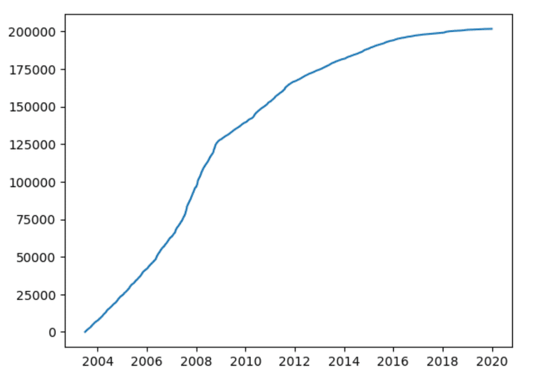

$${\tau=1e-5}$$で固定ウィンドウ法により定常になる、最小の$${d, d\in [0,2]}$$を求める。

def plotMinFFD(process,WindowWidth,thres,dmin=0.,dmax=1.,dnum=21):
    from statsmodels.tsa.stattools import adfuller
    '''
    Finding the minimum differentiating factor that passes the ADF test
    
        Parameters:
            process (np.ndarray): array with random process values
            WindowWidth (bool): flag that shows whether to use fixed width window (if True)
                                         or expandingi width window (if False)
            thres (float): threshold for cutting off weights
    '''
    out = pd.DataFrame(columns=['adfStat', 'pVal', 'lags', 'nObs', '95% conf'], dtype=object)
    printed = False
    
    for d in np.linspace(dmin, dmax, dnum):
        if WindowWidth: #Fixed Window
            process_diff = fracDiff_FFD(pd.DataFrame(process), d, thres)
        else:           #Entending Window
            process_diff = fracDiff(pd.DataFrame(process), d, thres)    
        test_results = adfuller(process_diff, maxlag=1, regression='c', autolag=None)
        out.loc[d] = list(test_results[:4]) + [test_results[4]['5%']]
        if test_results[1] <= 0.05 and not printed:
            print(f'Minimum d required: {d}')
            d_min=d
            printed = True
    fig, ax = plt.subplots(figsize=(11, 7))
    ax.plot(out['adfStat'])
    ax.axhline(out['95% conf'].mean(), linewidth=1, color='r', linestyle='dotted')
    ax.set_title('Searching for minimum $d$')
    ax.set_xlabel('$d$')
    ax.set_ylabel('ADF statistics')
    plt.show()
    return d_min, out

d,outADF=plotMinFFD(logClose,True,1e-5,dmin=0.0,dmax=2.,dnum=41)

$${d=2}$$で差分を取り、定常となった時系列と、対数累積時系列の相関を取る。

lCFFD = fracDiff_FFD(logClose, d=2.0, thres=1e-5).dropna()
df=(pd.DataFrame()
    .assign(org=close)
    .assign(log=logClose)
    .assign(ffd=lCFFD['Close'])
    ).dropna()
df.corr()

差分し、定常となった時系列と、オリジナル時系列、対数累積時系列の間に相関はない。
　次に、共和分検定を行う。

def printEGcoint(p0,p1):
    from statsmodels.tsa.stattools import coint
    # pVal<0.05 has cointegration
    EGcoint = coint(p0, p1)
    print('T-statistic:', EGcoint[0])
    print('p-value:', EGcoint[1])
    print('Critical Values:')
    critical_value_labels = ['1%', '5%', '10%']
    for i, value in enumerate(EGcoint[2]):
        print('\t%s: %.3f' % (critical_value_labels[i], value)) 

　この検定を行う前に、二つの時系列が共和分を持つ条件は、二つともが単位根を持つことを確かめる。
　また、statsmodelsのcoint関数は、与えられた二つの時系列$${y_0}$$、$${y_1}$$について、共和ベクトル$${(a,b)}$$を用いた線型結合$${ay_0 + b y_1}$$の定常性の計算に最小二乗法を使っていることで、
$${coint(x,y}$$と$${coint(y,x)}$$では答えが違うことがある。
　これを、単位根のあるオリジナル時系列と対数累積時系列、定常時系列で単位根のない分数差分された時系列で見ていく。

printADF(df.org)
printADF(df.log)
printADF(df.ffd)

print('Dollar Bar vs. FFD')
printEGcoint(df.org, df.ffd)

print('Cumsum of LogPrice vs. FFD')
printEGcoint(df.log, df.ffd)


print('Cumsum of LogPrice vs. Dollar Bar')
printEGcoint(df.log, df.org)
printEGcoint(df.org, df.log)

帰無仮説「共和分を持たない」は、すべての組み合わせで受け入れられているが、ADF検定で単位根を持たないと判定されている分数差分時系列FFDが入っている結果は適当ではないことに留意するべきである。
　ここに反例として、分数差分時系列とドルバーの順序を逆にして共和分検定を行った結果を示す。

「共和分を持たない」帰無仮説は棄却され、共和分を持つ結果となっている。先ほど見た通りに、分数差分された時系列には単位根はない。したがって、この結果で、共和分を持つと結論づけることは間違いである。

差分された時系列にJarque-Bera正規性検定を行う

Jarque-Bera正規性検定の帰無仮説「与えられたデータは正規分布に従う」はp値0.0で棄却されている。よって、差分時系列は正規性を持たない。