固定幅ウィンドウを使った分数次差分は、許容値$${\tau}$$を下回る、$${\tau \le |w_k^*|、\tau > |w_{k^*+1}|}$$となる、$${k^*}$$後の重みをゼロにする。
$${\tilde{w_k} = \left\{ \begin{array}{ll} w_k & (k \le k^*)\\ 0 & (k \gt k^*)\end{array}\right.}$$

よって、時系列は、$${\{X_t\}, t=T-k^*+1, T-k^*+2, \dots T}$$について、
$${\tilde{X_t}=\sum^{k^*}_{k=0}\tilde{w_k} X_{t-k}}$$となる。
　固定ウィンドウ法では、拡大ウィンドウ法とは違い、$${\{\tilde{X_t}\},t=k^*,k^*+1, \dots T}$$で同じ重みのベクトルを使うので、重みを足されることによる負のドリフトが発生しない。
　固定ウィンドウ方の実装はスニペット5.3で与えられている。

def getWeights_FFD(d, thres):
    '''
    Computing the weights for differentiating the series with fixed window size

    '''
    w,k=[1.],1
    while True:
        w_ = -w[-1]/k*(d-k+1)
        if abs(w_) < thres:
            break
        w.append(w_); k+=1
    return np.array(w[::-1]).reshape(-1,1)

def fracDiff_FFD(series, d, thres=1e-5):
    '''
    Fractional differentiation with constant width window
    '''
    w, df = getWeights_FFD(d, thres), {}
    width = len(w)-1
    for name in series.columns:
        seriesF,df_=series[[name]].ffill().dropna(),pd.Series(dtype='float64')
        for iloc in range(width, seriesF.shape[0]):
            loc0, loc1 = seriesF.index[iloc - width], seriesF.index[iloc]
            if not np.isfinite(series.loc[loc1,name]): continue
            df_[loc1]=np.dot(w.T,seriesF.loc[loc0:loc1])[0,0]
        df[name]=df_.copy(deep=True)
    df=pd.concat(df,axis=1)
    return df

　この方法を、拡大ウィンドウ法と同じくE-mini S&P500先物ドルバーに適用する。

close = Dbar['Close'].to_frame()
FWfd = fracDiff_FFD(close, d=0.4, thres=1e-4)
FWd0 = pd.DataFrame(index=close.index).assign(Close = close, FixW_t1e_4 = ffd)
FWd0[['FixW_t1e_4', 'Close']].plot(secondary_y='Close',figsize=(10,8))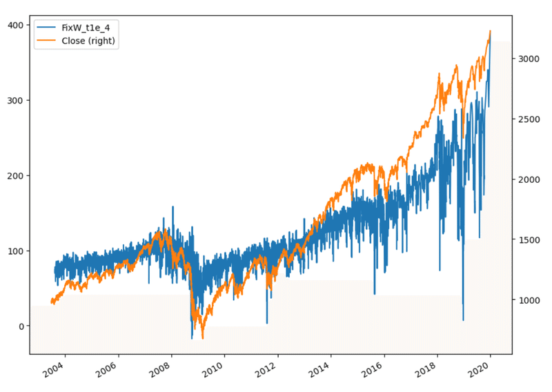

メモリーを保持した定常性

非定常の時系列に固定ウィンドウ法で分数次差分をとり、ADF検定によって単位根を持たない（すなわち定常）であると判定される最小の分数次$${d^*}$$を求められる。
　この$${d^*}$$は定常性を得るために除去される最小のメモリー量と解釈できる。
$${\{X_t\}}$$が定常であるなら、$${d^*=0}$$
$${\{X_t\}}$$が単位根を持つなら、$${d^*<1}$$
$${\{X_t\}}$$が発散を持つならば、$${d^*>1}$$
差分をとらなければならないのが、$${0< d^* << 1}$$の穏やかな非定常の場合であるが、整数次差分を取ると過剰にメモリーを取り除いてしまう。よって、$${0<d<1}$$の範囲で、定常となる$${d}$$を見つけることが望ましい。最小の$${d}$$を見つけるコードはスニペット5.4で与えられている。

def plotMinFFD(process,WindowWidth,thres):
    from statsmodels.tsa.stattools import adfuller
    '''
    Finding the minimum differentiating factor that passes the ADF test
    
        Parameters:
            process (np.ndarray): array with random process values
            WindowWidth (bool): flag that shows whether to use fixed width window (if True)
                                         or expandingi width window (if False)
            thres (float): threshold for cutting off weights
    '''
    out = pd.DataFrame(columns=['adfStat', 'pVal', 'lags', 'nObs', '95% conf'], dtype=object)
    printed = False
    
    for d in np.linspace(0, 1, 21):
        if WindowWidth: #Fixded  Window
            process_diff = fracDiff_FFD(pd.DataFrame(process), d, thres)
        else:           #Extend  Window
            process_diff = fracDiff(pd.DataFrame(process), d, thres)    
        test_results = adfuller(process_diff, maxlag=1, regression='c', autolag=None)
        out.loc[d] = list(test_results[:4]) + [test_results[4]['5%']]
        if test_results[1] <= 0.05 and not printed:
            print(f'Minimum d required: {d}')
            d_min=d
            printed = True
    
    fig, ax = plt.subplots(figsize=(11, 7))
    ax.plot(out['adfStat'])
    ax.axhline(out['95% conf'].mean(), linewidth=1, color='r', linestyle='dotted')
    ax.set_title('Searching for minimum $d$')
    ax.set_xlabel('$d$')
    ax.set_ylabel('ADF statistics')
    plt.show()
    return d_min,out

分数次差分を使った特徴量変換は、差分が取れるように、時系列の累積を取り、$${d\in[0,1]}$$の$${d}$$に対してFFD(d)系列を計算し、ADF統計量のp値が5％を下回る最小のdを求め、これから予測に用いる特徴量のFFD時系列を作成する。