Introducing Expected Threat (xT)
Modelling team behaviour in possession to gain a deeper understanding of buildup play.
Karun Singh (@karun1710)

When in possession...

One simplified way of viewing buildup play is as follows: when a team has possession in a certain position, they can either shoot (and score with some probability), or move the ball to a different location via a pass or a dribble. This continues until the team either loses possession, or scores a goal.

ビルドアッププレーを表示するための簡単な方法の1つは次の通りである。チームが特定の位置でポゼッションしているとき、シュートする（そしてある確率で得点する）か、パスかドリブルでボールを別の場所に動かすことができる。これは、チームがポゼッションを失うか、得点を決めるまで続く。

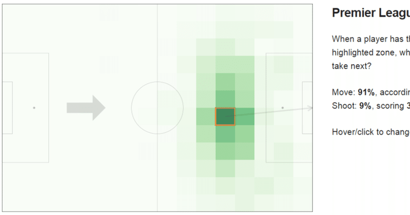
If we run with this simplified model of buildup play, what does the data look like? From each position, how often do players shoot (and how often do they score?), how often do they move the ball, and where do they move it to? The following visualization aggregates data over a whole season (2017-18) of Premier League games, go ahead and explore how players behave by clicking on different zones!

この単純化されたビルドアップモデルで実行した場合、データはどのようになるか。各位置から、選手はどのくらいの頻度でシュートし（そしてどのくらいの頻度で得点し）、どのくらいの頻度でボールを動かし、そしてどこにボールを動かすか。次の視覚化は、プレミアリーグの全2017-18シーズンにわたるデータをまとめたもので、さまざまなゾーンをクリックして選手のアクションを探ろう。

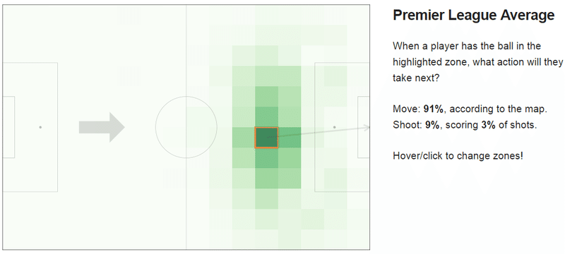
After playing around with this view of the data, you should begin to see that every zone location (x, y) has certain attributes:

このデータビューで試した後、すべてのゾーン位置(x,y)に特定の属性があることを確認し始めよう。

- Move probability m(x,y): when a player has possession in zone (x,y), how often do they opt to move (i.e. pass or dribble) the ball as their next action?
- Shoot probability s(x,y): when a player has possession in zone (x,y), how often do they opt to shoot as their next action? In our simplified universe, players can only either move or shoot, so by definition m(x,y)+s(x,y)=100%.
- Move transition matrix T(x,y): in the cases where the player moves from zone (x,y), what is the probability that they move to each of the other zones? The visualization above shows these probabilities in shades of green.
- Goal probability g(x,y): in the cases where the player shoots from zone (x,y), what is the probability that the shot turns into a goal? Note that this quantity is essentially a very simple implementation of xG!

- 移動確率m(x,y)：選手がゾーン(x,y)でポゼッションしているとき、次のアクションとしてどのくらいの頻度でボールを移動（すなわちパスまたはドリブル）させるか。
- シュート確率s(x,y)：選手がゾーン(x,y)でポゼッションしているとき、次のアクションとしてどれぐらいの頻度でシュートを選ぶか。単純化された世界では、選手は移動またはシュートしかできないので、定義上m(x,y)+s(x,y)=100%である。
- 移動遷移行列T(x,y)：選手がゾーン(x,y)から移動した場合、他の各ゾーンに移動する確率はどのくらいか。上の視覚化は、これらの確率を緑色の濃淡で示す。
- 得点確率g(x,y)：選手がゾーン(x,y)からシュートした場合、シュートが得点になる確率はどのくらいか。この量は本質的にxGの非常に単純な実装である。

Note: for the purposes of this simplified model, we consider only 'successful' moves, i.e. moves that were completed without possession being lost. You could, quite easily, consider all attempted moves as well, though at the cost of making your model slightly more complex (and harder to concisely explain in a blog post!).

注：この単純化されたモデルの目的のために、「成功した」移動、すなわちポゼッションを失うことなく完了した移動のみを考慮する。モデルをやや複雑にするという代償を払って（およびブログ記事で簡潔に説明するのはより難しくなるが）、比較的簡単に、すべての試行された移動も同様に検討することができる。

Another note: if you have a quantitative background, this might remind you of a Markov model where each grid location is a state, and passing or dribbling leads to state transitions.

別注：もし統計学的な背景を持つ場合、これは各グリッド位置が状態であり、パスまたはドリブルが状態遷移につながるマルコフモデルを思い出させる。

Looking beyond checkmate

Now that we have some notation, let's recap what we're trying to do here. The problem with purely shot-based models like xG when it comes to analyzing buildup play is that many meaningful actions don't result in good shooting positions immediately, but rather lead to good shooting positions multiple actions later. This idea is put forth very eloquently by Cervone et al. in the context of basketball analytics (although this quote is surprisingly transferable to football).

ここでいくつかの表記法があるので、ここでやろうとしていることを要約しよう。ビルドアッププレーの分析に関してxGのような純粋なシュートベースのモデルを使用する場合の問題は、多くの意味のあるアクションがすぐには良いシュート位置にならず、複数のアクションの後になるということである。この考えは、バスケットボール分析の文脈でCervone氏らによって非常に雄弁に提示されている（ただしこの引用は驚くほどフットボールに譲渡可能である）。

"Despite many recent innovations, most advanced metrics remain based on simple tallies relating to the terminal states of possessions like points, rebounds, and turnovers. While these have shed light on the game, they are akin to analyzing a chess match based only on the move that resulted in checkmate, leaving unexplored the possibility that the key move occurred several turns before. This leaves a major gap to be filled, as an understanding of how players contribute to the whole possession – not just the events that end it – can be critical in evaluating players, assessing the quality of their decision-making, and predicting the success of particular in-game tactics."

「最近の多くの技術革新にもかかわらず、最も先進的な指標は、ポイント、リバウンド、およびターンオーバーのようなポゼッションの最終状態に関する単純な集計に基づいている。これらはゲームに光を当てたが、彼らはチェックメイトをもたらした動きだけに基づいてチェスの試合を分析することに似ていて、重要な動きが数ターン前に起こった可能性を未踏のままにした。選手が（最後のイベントだけでなく）ポゼッション全体にどのように貢献しているかを理解することは、選手の評価、意思決定の質の評価、および特定のゲーム内戦術の成功の予測において重要になる可能性があるため、埋めるべき大きなギャップを残す。」

So how can we look beyond checkmate given the data that we have? How can we assign values to zones that reflect not just their immediate shooting value, but the future rewards they can bring (through movements of the ball to other zones)? The key intuition here is that when you have possession in zone (x,y), you have a choice: you can either shoot and score with some probability, or you can move the ball to a different location. Given this background, we can formulate the problem as follows.

それでは、持っているデータを考えると、どのようにしてチェックメイトを越えて見ることができるか。即座のシュート価値だけでなく、（他のゾーンへのボールの移動を通しての）将来の報酬を反映するゾーンにどのように値を割り当てることができるか。ここでの重要な直感は、あなたがゾーン(x,y)でポゼッションしているとき、選択肢があるということである。シュートしてある確率で得点することも、別の場所にボールを移動させることもできる。このような経緯から、問題は次のように定式化できる。

Note: admittedly, the next couple of sections get quite technical (though I've tried to break down the math as much as possible). Although I'd strongly recommend reading through them, if you'd prefer to skip these and jump to the results of the model, click here.

注：確かに、次の数セクションはかなり技術的になる（ただしできる限り数学を分割するようにした）。読み進めることを強くお勧めするが、これらをスキップしてモデルの結果にジャンプする場合は、ここをクリックしよう。

Deriving xT

Note: for the purposes of this post, we're working with a 16x12 grid on the pitch, which gives us 192 zones. In practice, you can choose a different resolution based on how much data you have!

注：この記事の目的のために、ピッチの16x12グリッドを使って作業し、これにより192ゾーンが得られる。実際には、データ量に基づいて異なる解像度を選択できる。

Let V(x,y) be the 'value' that our algorithm assigns to zone (x,y).
Now imagine you have the ball at your feet in zone (x,y). You have two choices: shoot, or move the ball.
Based on past data, we know that whenever you shoot from here, you will score with probability g(x,y). Thus, if you shoot, your expected payoff is g(x,y).

V(x,y)をアルゴリズムがゾーン(x,y)に割り当てる「値」とする。
今、自分の足元にボールがゾーン(x,y)にあると想像する。2つの選択肢、シュートかボールを動かす。
過去のデータに基づいて、ここからシュートたびに確率g(x,y)で得点することを知っている。従ってシュートした場合、期待値はg(x,y)である。

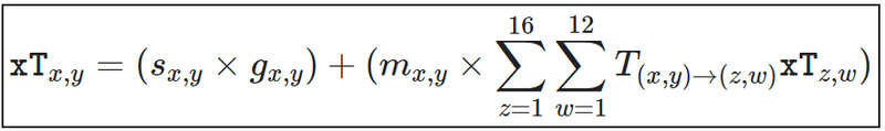
Or, you can opt to move the ball via a pass to a teammate or by dribbling it yourself. But there's another choice to make here: which of the 192 zones should you move it to? Say you choose to move the ball to some new zone, (z,w). In this case, your expected payoff is the value at zone (z,w), i.e. V(z,w). But this was just one of the 192 choices that you had; how can we compute the expected payoff for all of the 192 choices in totality? Here's where the move transition matrix T(x,y) comes in: based on past data, we know where you're likely to move the ball to whenever you're in zone (x,y), so we can proportionally weight the payoffs from each of the 192 zones. Specifically, for each zone (z,w), the payoff is T(x,y)→(z,w)×V(z,w), i.e. the probability of moving to that zone times the reward from that zone. To get the total expected payoff for moving the ball, we must sum this quantity over all possible zones:

または、味方へのパスか、自分でドリブルすることによってボールを移動することを選択できる。しかし、ここで他に選択することがある。192のゾーンのどれに移動するべきか。ボールを新しいゾーン(z,w)に移動することを選択したとする。この場合、期待値はゾーン(z,w)の値、つまりV(z,w)である。しかし、これは192の選択肢のうちの1つにすぎない。全部で192の選択肢のすべてに対する期待値をどのように計算できるか。移動遷移行列T(x,y)は次のようになる。過去のデータに基づいて、ゾーン(x,y)にいるときはいつでもボールをどこに移動させる可能性があるかがわかっているので、各192ゾーンからの報酬に比例して重み付けできる。具体的には各ゾーン(z,w)について、報酬はT(x,y)→(z,w)×V(z,w)、すなわちそのゾーンに移動する確率×そのゾーンからの報酬である。ボールを動かすことで予想される総報酬を得るために、全ての可能なゾーンにわたってこの量を合計しなければならない。

Finally, let's piece it all together. We computed the payoff if you shoot as g(x,y), and the payoff if you move the ball as ∑∑T(x,y)→(z,w)×V(z,w). Based on past data, we know that you tend to shoot s(x,y) percent of the time, and you opt to move the ball m(x,y) percent of the time. Therefore, let's weight these two outcomes based on the probability of each of them happening, to obtain our final value for zone x,y:

最後に、全部まとめてみる。g(x,y)としてシュートした場合の報酬を計算し、ボールを動かした場合の報酬を∑∑T(x,y)→(z,w)×V(z,w)として計算した。過去のデータに基づいて、s(x,y)%でシュートを放つ傾向があり、m(x,y)%でボールを動かすのを選ぶことを知っている。したがって、これら2つの結果のそれぞれが発生する確率に基づいて重み付けして、ゾーン(x,y)の最終値を取得する。

This quantity looks beyond the checkmate; it values locations based on not just the immediate shooting threat, but the potential to induce danger later in the possession sequence. It is inherently designed to capture a notion of 'threat', so 'Expected Threat' (xT) seems like an apt name for it. Of course, the naming process wouldn't be complete without rewriting the whole equation again in a box with the updated variable name:

この量はチェックメイトを超えて見える。それは即座のシュートの脅威だけではなく、ポゼッション連鎖の後半で危険を引き起こす可能性に基づいて位置を評価する。それは本質的に「脅威」の概念をとらえるように設計されているので、「脅威期待値」（xT）はそれに対する適切な名前のように思える。もちろん、命名プロセスは、更新された変数名のボックスに方程式全体を再度書き直さなければ完了しない。

But wait, there's more...

Unfortunately that formula on its own is buggy without one additional detail. If you look at the formula carefully, you'll see that it is flawed since computing the xT value for some zone (x,y) requires that we already know the xT value for all the other zones. But all the other zones also suffer from the exact same flaw, so this forms a cyclic dependency that we can't theoretically resolve!

残念ながら、その公式はそれ自体では1つの追加の詳細がないとバグがある。公式を注意深く見ると、あるゾーン(x,y)のxT値を計算するには、他のすべてのゾーンのxT値がわかっている必要があるため、この式に欠陥があることがわかる。しかし、他のすべてのゾーンもまったく同じ欠陥に悩まされているため、これは循環的な依存関係を形成し、理論的には解決できない。

Fortunately, in practice there is a neat workaround. All we need to do is start off with xT(x,y)=0 for all zones (x,y), and evaluate this formula not once, but iteratively until convergence. During each iteration, we evaluate the new xT for each zone by using xT values from the previous iteration. Empirically, I found 4-5 iterations to be sufficient for reasonable convergence, though this may vary based on your dataset.

幸い、実際にはきちんとした回避策がある。必要なのは、すべてのゾーン(x,y)に対してxT(x,y)=0から始め、この式を一度だけではなく収束まで反復して評価することである。各反復中に、前の反復からのxT値を使用して、各ゾーンの新しいxTを評価する。経験的に、合理的な収束には4〜5回の反復で十分であることがわかったが、これはデータセットによって異なる場合がある。

Besides breaking the cyclic dependency and leading to convergence, this process comes with another added benefit: interpretability. Let's take a step back and think about what happens at iteration 1. At this point, we are using our initialization of xT = 0 for all zones. Here's what happens to our xT formulation:

このプロセスには、循環的な依存関係を解消して収束につながること以外にも、次のような利点がある。解釈可能性だ。一歩戻り、反復1で何が起こるかを考えてみる。この時点では、すべてのゾーンに対してxT=0の初期化を使用している。これがxT定式化に起こることである。

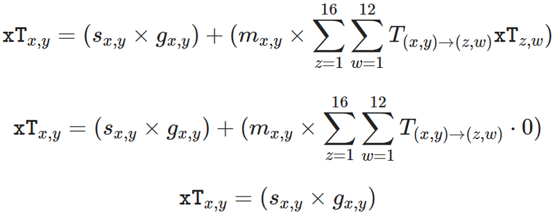
While not exactly xG, you can think of this as a value that represents how good a shooting position (x,y) is. In other words, after iteration 1, we essentially have an xG model! An alternative way to think about this is that at iteration 1, we are only allowing the checkmate: we are valuing positions as though shooting was the only option, and passing and dribbling did not exist.

正確にはxGではないが、これはシュート位置(x,y)の良さを表す値と考えることができる。言い換えれば、反復1の後、本質的にxGモデルを手に入れたことになる。これについて考える別の方法は、反復1ではチェックメイトのみを許可している。シュートが唯一の選択肢であるかのように位置を重視しており、パスとドリブルは存在しない。

Now, in the second iteration, the new xT computation will use the xT values that were computed in iteration 1. At this point, the 'move' term in the formula will no longer be 0. This effectively means that we are now considering the possibility of "move, then shoot" in addition to just "shoot". We are now looking one move before the checkmate.

さて、2回目の反復では、新しいxT計算は反復1で計算されたxT値を使用する。この時点で、公式の「移動」項は0にならない。これは事実上、がただ「シュートする」だけでなく「移動してからシュートする」可能性を現在検討していることを意味する。今チェックメイトの前の1つの動きを見ている。

The same logic can be extended for multiple steps; for example, in the third iteration, we are additionally considering the possibility of "move, move, shoot" and looking up to two moves before the checkmate. This idea is powerful because it lends a very interpretable meaning to xT. Rather than being a score on an arbitrary scale, it has a very natural meaning (just like its distant cousin, xG). Specifically, xT(x,y) at iteration n represents the probability of scoring within the next n actions.

同じ論理を複数のステップに拡張できる。たとえば、3回目の反復では、「移動、移動、シュート」の可能性をさらに検討し、チェックメイトの前に最大2つの移動を見る。この考えはxTに非常に解釈しやすい意味を与えるので強力である。任意のスケールのスコアではなく、（遠いいとこxGのように）非常に自然な意味を持つ。具体的には、反復nにおけるxT(x,y)は、次のn個の動作内で得点する確率を表す。

Visualizing xT

Now that we have a way to find xT across the pitch, what does the end result look like? The visualization below shows a 2D as well as a 3D representation of the value surface generated by xT, using events across all the matches of the 2017/18 Premier League season. Use the slider to view the xT at different iterations within the algorithm, and hover/click to change zones on the pitch!

ピッチ全体でxTを求める方法ができたので、最終結果はどのようになるか。以下の視覚化は、2017/18プレミアリーグシーズンのすべての試合にわたるイベントを使用して、xTによって生成された価値面の2Dおよび3D表現を示す。スライダーを使用してアルゴリズム内のさまざまな反復でxTを表示し、ホバーまたはクリックしてピッチ上のゾーンを変更できる。

As you step through the successive iterations, it's worth noticing some interesting things:
- At iteration 0, the map is flat since we initialize xT = 0 for all zones to begin with.
- At iteration 1, we have effectively computed an xG model.
- At each subsequent iteration, you can see the xT spread to areas further away from the goal (because, as explained above, each iteration essentially allows us to account for one more action in the buildup play).
- The xT values begin to converge (to a reasonable degree) after 4-5 iterations.

連続した反復が進むにつれ、いくつかの興味深いことに気づく価値がある。
- 反復0では、すべてのゾーンでxT=0で初期化するため、マップは平坦である。
- 反復1では、xGモデルを効果的に計算した。
- その後の反復ごとに、xTがゴールからより離れた領域に広がるのがわかる（なぜなら上で説明したように、各反復は本質的にビルドアッププレーのもう1つのアクションを説明するのを可能にするため）。
- xT値は、4〜5回の反復後に（妥当な程度まで）収束し始める。

Applying xT

Zooming out a bit, the point of xT was to come up with a metric that can quantify threat at any location on the pitch. Now that we have xT, we can value individual player actions in buildup play by computing the difference in xT between the start and end locations. In other words, we will say that an action that moves the ball from location (x,y) to location (z,w) has value xT(z,w)−xT(x,y). Once again, there is a nice interpretable meaning to this: the value of an action is equal to the % change in the team's chances of scoring in the next 5 actions due to the action (note that here we're using the xT computed after 5 iterations, hence 'next 5 actions').

xTのポイントは、少しズームアウトすると、ピッチ上の任意の場所で脅威を定量化できる指標を考え出すことだった。xTができたので、開始位置と終了位置の間のxTの差を計算することによって、ビルドアッププレーにおける個々の選手のアクションを評価できる。言い換えれば、位置(x,y)から位置(z,w)へボールを移動させるアクションは値xT(z,w)−xT(x,y)を有すると言うことになる。繰り返しになるが、これには良い解釈可能な意味がある。あるアクションの価値は、そのアクションに起因する次の5つのアクションにおけるチームの得点機会の％変化に等しい（ここでは5回の反復後に計算されたxTを使用しているため、「次の5つのアクション」となる）。

Now, let's try answering the Kolašinac-Özil credit assignment problem from before using the xT framework:
1. Özil's pass takes the ball from xT = 0.077 to xT = 0.158. Difference in xT due to Özil = 0.081.
2. Kolašinac's pass takes the ball from xT = 0.158 to xT = 0.171. Difference in xT due to Kolašinac = 0.013.
Looking at these numbers, Özil is responsible for 0.081/(0.081+0.013)=86% of the net change in xT, so the framework would attribute 86% of the credit to him and 14% to Kolašinac.

それでは、xTフレームワークを使用して前述のコラシナツとエジルの報酬割り当て問題に答えよう。
1. エジルのパスはxT = 0.077からxT = 0.158へボールを送る。エジルによるxTの差は0.081である。
2. コラシナツのパスはxT = 0.158からxT = 0.171へボールを送る。コラシナツによるxTの差は0.013である。
これらの数値を見ると、エジルはxTの正味変化の0.081/(0.081+0.013)=86％を占めているため、フレームワークは報酬の86％をエジルに、14%をコラシナツに割り当てる。

Note: for simplicity, in this example I've discretized start and end locations to the grid cell that they fall in. However, if you're doing some kind of sophisticated analysis where precision matters a lot, you might want to use bilinear interpolation. You can still compute the xT map using a fixed-size grid, but when computing values for events, you can use the exact location coordinates to get more precise estimates!

注：簡略化のために、この例では開始位置と終了位置をそれらが入るグリッドセルに離散化した。ただし、精度が非常に重要となるような高度な分析を行う場合は、バイリニア補間を使用することを勧める。固定サイズのグリッドを使用してxTマップを計算することはできるが、イベントの値を計算するときは、正確な位置座標を使用してより正確な推定値を取得できる。

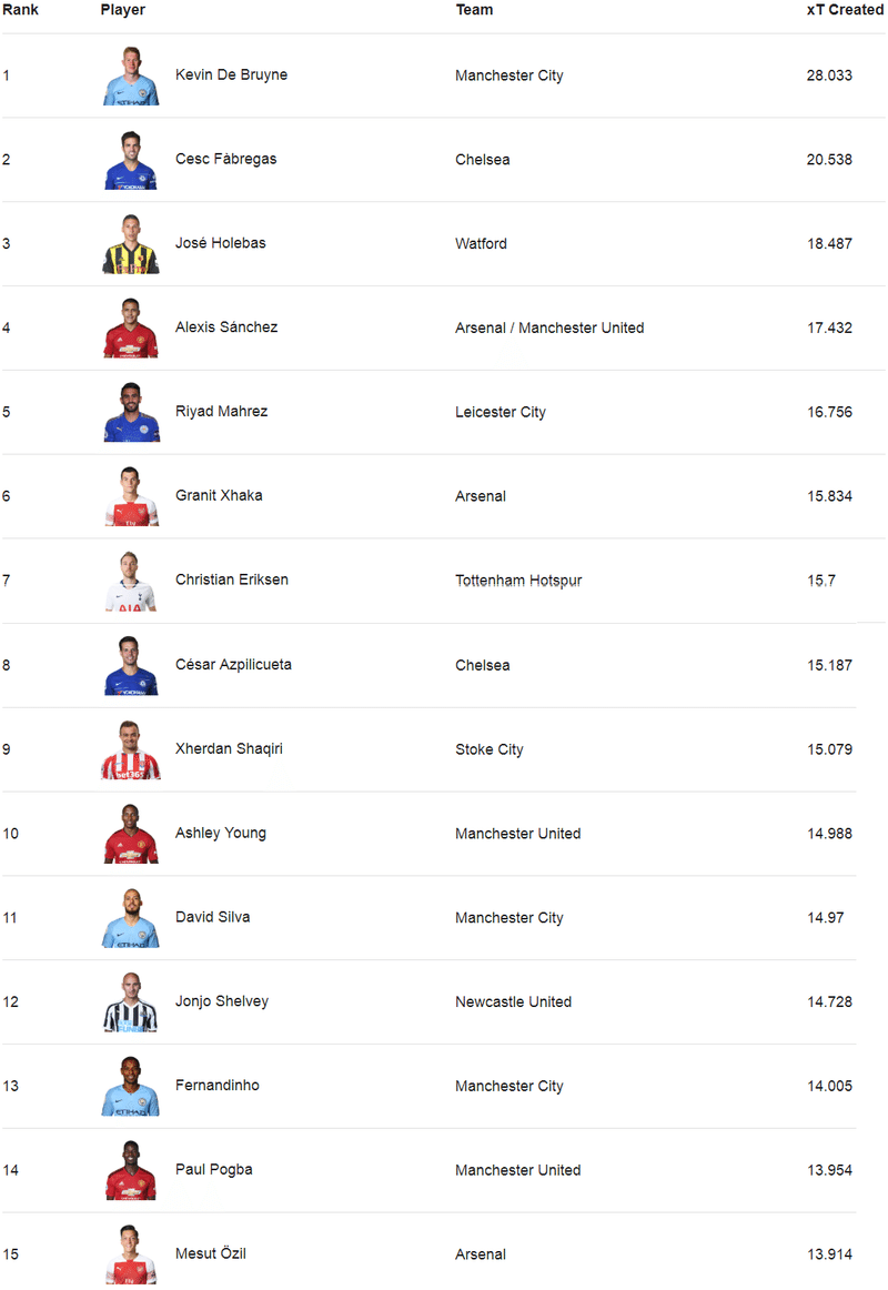
Top xT creators

As a sanity check, let's also look at the top xT creators during the 2017/18 Premier League season. The table below shows the top 15 players in the league whose actions created the highest cumulative change in xT. Note that this is not normalized by the number of actions taken – it is based on the raw sum of xT created. This is intentional, because it surfaces players who not only know how to create danger, but those who do it consistently at a high volume. The inclusion of Holebas at #3 might surprise you, but the left-back has established himself as Watford's most consistent and most dangerous creator.

健全性チェックとして、2017/18プレミアリーグシーズン中のxT創造者上位も見よう。以下の表は、xTの累積変化が最も大きかったリーグの上位15選手を示す。これはアクション数によって正規化されておらず、xTの生の合計に基づくことに注意する。危険を生み出す方法を知るだけでなく、常に大量に危険を冒している選手を浮上させるので、これは意図的である。ヨゼ・ホレバスが含まれることは驚きかもしれないが、左DFの彼がワトフォードの最も一貫性があり最も危険な創造者としての地位を確立した。

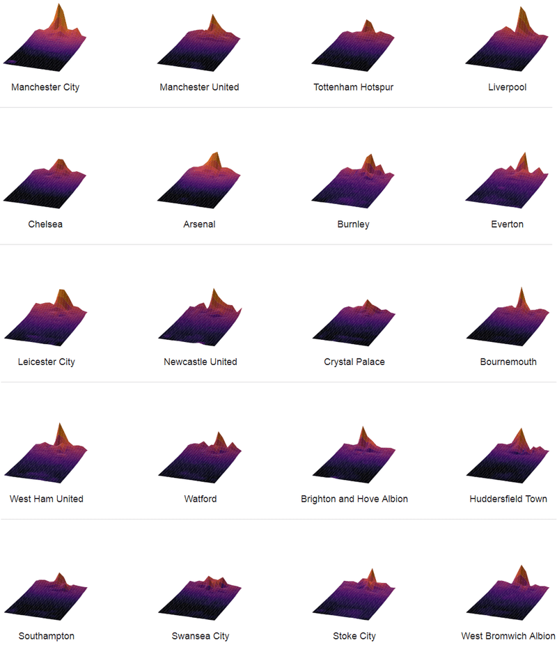
Besides simple credit assignment in buildup play, the xT framework opens the door for a host of other applications. For example, so far I've only shown xT results using an entire season's worth of Premier League data: but of course, this means we lose team-specific information. There's no doubt that teams behave differently in possession, prioritizing different areas of the pitch and exploiting different paths to goal based on their strengths (and weaknesses). What happens if, instead of clubbing all the Premier League teams into one analysis, we compute xT on a per-team basis?

ビルドアッププレーでの単純な報酬割り当てに加えて、xTフレームワークは他の多くの応用への扉を開く。たとえばこれまでのところ、シーズン全体のプレミアリーグのデータを使用してxTの結果を表示しただけである。しかしもちろん、これはチーム固有の情報を失うことを意味する。チームがそれぞれ異なる強み（および弱み）に基づいてピッチのさまざまなエリアを優先し、ゴールへのさまざまな経路を選択して、ポゼッションの動作が異なることは間違いない。すべてのプレミアリーグのチームを1つの分析にまとめるのではなく、チームごとにxTを計算するとどうなるか。

Visualizing per-team xT

Note: reminder that this is based on data from the 2017/18 season and not the current season!

注：これは2017/18シーズンのデータであり、現在のシーズンではないことに注意する。

Sure enough, we do see a lot of variance across different teams. In addition to changes in the shape of the xT curve, note the differences in height. For instance, the shape of Manchester City and Spurs' curves are similar (which means they value the ball in similar areas of the pitch), yet their xT magnitudes are very different. This tells us that given the ball in the same position, City are much more threatening than Spurs (due to their higher conversion rate of possessions into goals).

案の定、チームによってさまざまな違いがある。xT曲線の形の変化に加えて、高さの違いに注意する。たとえば、マンチェスター・シティとスパーズの曲線の形状は似ているが（つまりピッチの同じ領域でボールを評価していることを意味する）、xTの大きさは非常に異なる。これは、同じ位置にボールがあるとすると、シティはスパーズよりもはるかに脅威的なことを示す（ポゼッションから得点への変換率が高いため）。

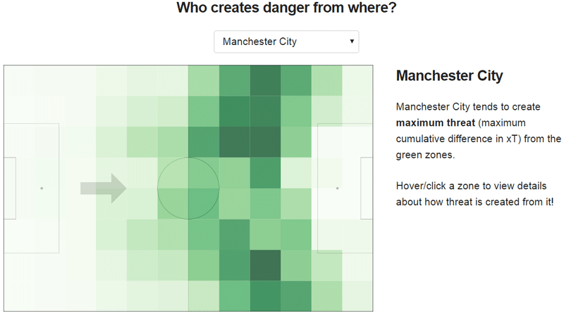
While these per-team xT maps are interesting to look at, they're not very actionable on their own. That being said, the underlying data is powerful because it can give us a team-specific view into how danger is created through buildup play. For example, one useful question to answer during pre-match analysis might be: where on the pitch do our opponents tend to create the most danger from?

これらのチームごとのxTマップは見てみるのは興味深いが、それだけでは実用的ではない。そうは言っても、基礎となるデータは強力で、なぜならビルドアッププレーによってどのように危険が生じるのかについてチーム固有の見解を得ることができるためである。たとえば、試合前の分析中に答える有用な質問の1つは次のようになる。相手がピッチ上のどこから最も脅威を与えているのか。

To answer this, we can use our opponent's xT map to value all of their actions from past matches, and aggregate these values based on the start location of the action. In other words, for each grid location, we can look at the actions that originated there, and sum the xT created by these actions. This will give us a per-location cumulative value that will highlight the amount of danger created from different areas of the pitch. Additionally, by highlighting the common end zones of actions starting in a particular zone, we can start to see our opponent's most dangerous passages of play. To make this even more useful for tactical preparation, we might want to also know who are the players that are responsible for creating threat through these passages.

これに答えるために、相手のxTマップを使用して過去の試合からの彼らの行動のすべてを評価し、アクション開始位置に基づいてこれらの値を集計することができる。言い換えれば各グリッド位置について、そこで発生したアクションを調べて、これらのアクションによって作られたxTを合計できる。これはピッチごとの異なるエリアから発生する脅威量を強調する位置ごとの累積値を与える。さらに、特定のゾーンで始まる共通の終了ゾーンのアクションを強調することで、相手の最も危険なプレーを見ることができる。これをさらに戦術的な準備に役立てるために、これらのプレーを通して脅威を生み出す責任を負っているのは誰であるかを知りたい。

The visualization below attempts to answer precisely these questions. The green map shows zones from where maximum xT is created. Hovering/clicking on a zone will show you the dangerous passages of play that originate there, as well as the players most responsible for them. Use the dropdown menu to switch to any other Premier League team!

以下の視覚化は、これらの質問に正確に答えようとする。緑色のマップは、xT最大値が作られた場所のゾーンを示す。ゾーンをホバー/クリックすると、そこで発生した危険なプレーと、それらに最も責任を負う選手が表示される。他のプレミアリーグのチームに切り替えるには、ドロップダウンメニューを使用する。

Future work

These were just a couple of applications of xT, and there are many more left to explore. The ability of xT to capture the on-the-ball behaviour of teams leads to several promising directions. Looking at how xT changes during the course of a possession sequence may help us, for example, in identifying and analyzing patterns of play such as counter-attacks. At the player level, we can assess an individual player's decision-making relative to how his team tends to play: "Is this player making high-reward passing choices given his team's xT profile? Would he be better off shooting rather than dribbling in certain areas?" Perhaps even more interesting is answering similar questions in the context of player scouting: "Can we tell if this player, who has never played for us, will fit into our system? Does he have a history of creating actions that will lead to high xT gains for us?"

これらはxTのほんの少しの応用で、そして探索すべきことがまだたくさんある。チームのオンザボールでのアクションを捕らえるxTの能力は、いくつかの有望な方向性を導く。例えば、カウンターアタックのようなプレーパターンを識別し分析する際に、ポゼッション連鎖の過程でxTがどのように変化するかを調べるのは有効かもしれない。選手レベルでは、チームがどのようにプレーする傾向があるかに関連して、個々の選手の意思決定を評価できる。「自分のチームのxTプロファイルを考えると、この選手は報酬の高いパスの選択をしているか。特定のエリアでドリブルをするよりも、シュートのほうが得策だろうか。」おそらくもっと興味深いのは、選手のスカウトの状況で同様の質問に答えることである。「これまでに一度もチームでプレーしたことのないこの選手が、このシステムに収まるかどうか。高いxT報酬をもたらすようなアクションを生み出した歴史があるか。」

If there are any directions that you're particularly excited about or want to explore together, please let me know! I'll continue to explore the limits of xT and will publish relevant results on my Twitter and on this blog.

特に興奮している、または一緒に探検したいという方向性があれば、知らせてほしい。xTの限界を探求し続け、そしてTwitterとこのブログで関連する結果を公表する。