Google Play ストアの評価するための 機械学習

はじめに
自己紹介:私立大学文系学部卒→メーカー約1年半→AIdemyのデータ分析を受講
今回はAIdemyを通じて学んだことをもとに機械学習アルゴリズムを使用して、Google Playストアのアプリの評価を予測します。
分析フロー
1.ライブラリのインポート
2.データのインプット
3.データの前処理
4.モデルの比較
まとめ
1.ライブラリのインポート
 #ライブラリのインポート
import pandas as pd
import numpy as np
import seaborn as sns
from sklearn import metrics
from sklearn.model_selection import train_test_split
import random
import matplotlib.pyplot as plt
%matplotlib inline
2.データのインプット
df = pd.read_csv('/content/googleplaystore.csv')3.データの前処理
df.info()出力
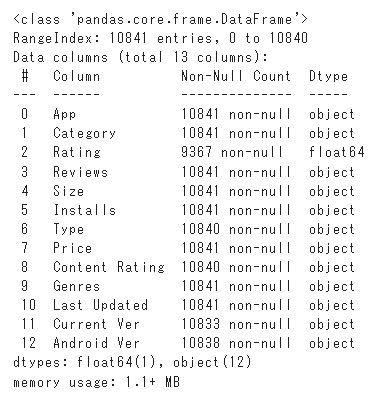
データを確認すると、対処する必要があるNull値は無く、私の目的は、アプリの評価を予測することなので、すべてのNaN値を削除します。
df.dropna(inplace = True)df.info()出力
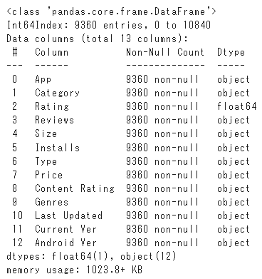
次の手順では、機械学習アルゴリズムでデータを処理するには、まずテキストから数値に変換する必要があります。
df.head()出力
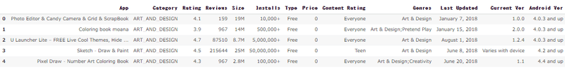
カテゴリ列から、各カテゴリを個別の番号に変換します。
# カテゴリを整数に処理
CategoryString = df["Category"]
categoryVal = df["Category"].unique()
categoryValCount = len(categoryVal)
category_dict = {}
for i in range(0,categoryValCount):
    category_dict[categoryVal[i]] = i
df["Category_c"] = df["Category"].map(category_dict).astype(int)
アプリのサイズをクリーニングし、欠損値を補完する。
 #scaling  and cleaning size of installation
def change_size(size):
    if 'M' in size:
        x = size[:-1]
        x = float(x)*1000000
        return(x)
    elif 'k' == size[-1:]:
        x = size[:-1]
        x = float(x)*1000
        return(x)
    else:
        return None

df["Size"] = df["Size"].map(change_size)
 #欠損値を補完する
df.Size.fillna(method = 'ffill', inplace = True)
インストール数の列をクリーニングする。
 #Cleaning  no of installs classification
df['Installs'] = [int(i[:-1].replace(',','')) for i in df['Installs']]
有料/無料の分類タイプをバイナリに変換する。
 #Converting  Type classification into binary
def type_cat(types):
    if types == 'Free':
        return 0
    else:
        return 1

df['Type'] = df['Type'].map(type_cat)
コンテンツ評価セクションを整数に変換します。
 #Cleaning  of content rating classification
RatingL = df['Content Rating'].unique()
RatingDict = {}
for i in range(len(RatingL)):
    RatingDict[RatingL[i]] = i
df['Content Rating'] = df['Content Rating'].map(RatingDict).astype(int)
機械学習アルゴリズムに不必要であると判断したため、これらの情報の一部を削除します。
 #無関係で不要なアイテムの削除
df.drop(labels = ['Last Updated','Current Ver','Android Ver','App'], axis = 1, inplace = True)
ジャンルのクリーニングを行う場合、ワンホットエンコーディングを適用する必要があります。しかし、第一に、それはカテゴリ別のサブセットであり、第二に、ダミー変数を適用すると独立変数の数が大幅に増加してしまいます。
代わりにこれに対処するために、そのようなジャンルデータを含む1つと除外する2つの別々の回帰を実行しました。データを含める場合、純粋に数値に基づいて、ジャンルセクションを介して提供される影響および情報のみを考慮します。
 #Cleaning  of genres
GenresL = df.Genres.unique()
GenresDict = {}
for i in range(len(GenresL)):
    GenresDict[GenresL[i]] = i
df['Genres_c'] = df['Genres'].map(GenresDict).astype(int)
フロートへのアプリの価格のクリーニング
 #Cleaning  prices
def price_clean(price):
    if price == '0':
        return 0
    else:
        price = price[1:]
        price = float(price)
        return price

df['Price'] = df['Price'].map(price_clean).astype(float)
最後に数値レビューの列を整数に変換します。
# レビューを数値に変換
df['Reviews'] = df['Reviews'].astype(int)df.info()出力
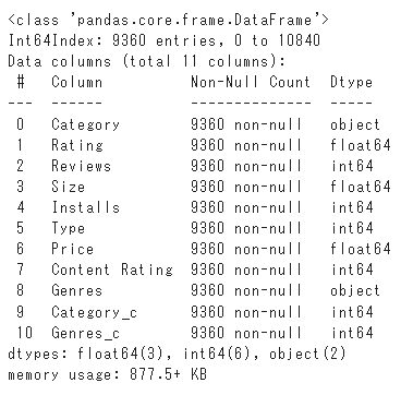
4.モデルの比較
dfとして定義されたカテゴリ変数の整数エンコーディングを持つデータフレームを最初に作成します。
df.head()df2として定義されたデータフレーム内の各カテゴリインスタンスのダミー値を具体的に作成した別のデータフレームを作成しました。
# エンコーディング用のカテゴリのダミー変数
df2 = pd.get_dummies(df, columns=['Category'])df2.head()出力

このインスタンスの目標は提供された既存のデータを使用できるかどうかを確認することです。(例:サイズ、レビュー数)はGoogleアプリケーションの評価を予測します。したがって、従属変数Yはアプリの評価になります。
注意すべき1つの重要な要素は、従属変数Yは離散変数と比較して連続変数であるということです。Yを離散変数に変換する方法は機械学習セッションの目的のためにYを連続変数として保持することにしました。
モデルに関しては、基本的には、線形回帰、SVR、およびRandom Forest回帰である3つのもっとも一般的なモデルを採用しました。
次に、予測結果を実際の結果とグラフィカルに比較してモデルを評価し、可能なベンチマークとして平均二乗誤差、平均絶対誤差、平均二乗対数誤差を使用します。
エラー言語の使用は、すべてのモデルを実行した後、最後に評価されます。
カテゴリ変数の処理に2つの異なる機能を持つ3つの回帰モデルを使用します。
以下は互換性のために、様々なモデルのエラー用語を取得するためのコードです。
 #for  evaluation of error term and
def Evaluationmatrix(y_true, y_predict):
    print ('Mean Squared Error: '+ str(metrics.mean_squared_error(y_true,y_predict)))
    print ('Mean absolute Error: '+ str(metrics.mean_absolute_error(y_true,y_predict)))
    print ('Mean squared Log Error: '+ str(metrics.mean_squared_log_error(y_true,y_predict)))
#エラー用語の評価をresults_indexに追加する 。
def Evaluationmatrix_dict(y_true, y_predict, name = 'Linear - Integer'):
dict_matrix = {}
dict_matrix['Series Name'] = name
dict_matrix['Mean Squared Error'] = metrics.mean_squared_error(y_true,y_predict)
dict_matrix['Mean Absolute Error'] = metrics.mean_absolute_error(y_true,y_predict)
dict_matrix['Mean Squared Log Error'] = metrics.mean_squared_log_error(y_true,y_predict)
return dict_matrix線形回帰モデル(ジャンルラベル無し)を見ることから始めます。
 #ジャンルラベルを除く
from sklearn.linear_model import LinearRegression
 #整数エンコーディング
X = df.drop(labels = ['Category','Rating','Genres','Genres_c'],axis = 1)
y = df.Rating
X_train, X_test, y_train, y_test = train_test_split(X, y, test_size=0.30)
model = LinearRegression()
model.fit(X_train,y_train)
Results = model.predict(X_test)
 #Creation  of results dataframe and addition of first entry
resultsdf = pd.DataFrame()
resultsdf = resultsdf.from_dict(Evaluationmatrix_dict(y_test,Results),orient = 'index')
resultsdf = resultsdf.transpose()
 #ダミーエンコーディング

X_d = df2.drop(labels = ['Rating','Genres','Category_c','Genres_c'],axis = 1)
y_d = df2.Rating
X_train_d, X_test_d, y_train_d, y_test_d = train_test_split(X_d, y_d, test_size=0.30)
model_d = LinearRegression()
model_d.fit(X_train_d,y_train_d)
Results_d = model_d.predict(X_test_d)
 #結果をresults  dataframeに追加する
resultsdf = resultsdf.append(Evaluationmatrix_dict(y_test_d,Results_d, name = 'Linear - Dummy'),ignore_index = True)plt.figure(figsize=(12,7))
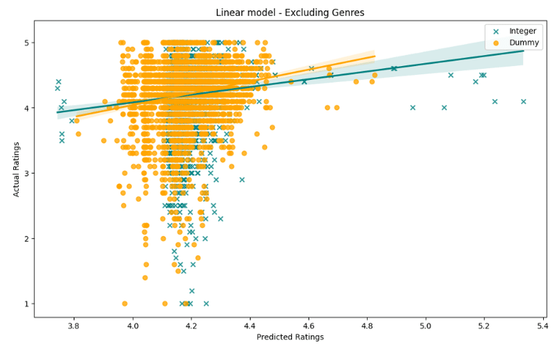
sns.regplot(x=Results,y=y_test,color='teal', label = 'Integer', marker = 'x')
sns.regplot(x=Results_d,y=y_test_d,color='orange',label = 'Dummy')
plt.legend()
plt.title('Linear model - Excluding Genres')
plt.xlabel('Predicted Ratings')
plt.ylabel('Actual Ratings')
plt.show()出力
print ('Actual mean of population:' + str(y.mean()))
print ('Integer encoding(mean) :' + str(Results.mean()))
print ('Dummy encoding(mean) :'+ str(Results_d.mean()))
print ('Integer encoding(std) :' + str(Results.std()))
print ('Dummy encoding(std) :'+ str(Results_d.std()))
出力
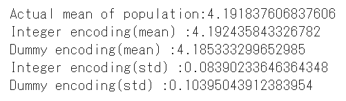
一見すると、予測精度の観点から、どのモデルが優れているかを実際に見るのは難しいです。しかし、印象的なのはダミーモデルは整数モデルと比較して低い評価の結果を好むようです。
予測結果の実際の平均を見ると、どちらもほぼ同じですが、ダミーエンコードされた結果は、整数エンコードされたモデルと比較して、はるかに大きな標準偏差を持っています。
次に数値としてジャンルラベルを含む線形モデルを見ていきます。
 #Including  genre label
 #整数エンコーディング
X = df.drop(labels = ['Category','Rating','Genres'],axis = 1)
y = df.Rating
X_train, X_test, y_train, y_test = train_test_split(X, y, test_size=0.30)
model = LinearRegression()
model.fit(X_train,y_train)
Results = model.predict(X_test)

resultsdf = resultsdf.append(Evaluationmatrix_dict(y_test,Results, name = 'Linear(inc Genre) - Integer'),ignore_index = True)
 #ダミーエンコーディング

X_d = df2.drop(labels = ['Rating','Genres','Category_c'],axis = 1)
y_d = df2.Rating
X_train_d, X_test_d, y_train_d, y_test_d = train_test_split(X_d, y_d, test_size=0.30)
model_d = LinearRegression()
model_d.fit(X_train_d,y_train_d)
Results_d = model_d.predict(X_test_d)

resultsdf = resultsdf.append(Evaluationmatrix_dict(y_test_d,Results_d, name = 'Linear(inc Genre) - Dummy'),ignore_index = True)plt.figure(figsize=(12,7))
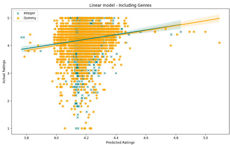
sns.regplot(x=Results,y=y_test,color='teal', label = 'Integer', marker = 'x')
sns.regplot(x=Results_d,y=y_test_d,color='orange',label = 'Dummy')
plt.legend()
plt.title('Linear model - Including Genres')
plt.xlabel('Predicted Ratings')
plt.ylabel('Actual Ratings')
plt.show()出力
print ('Integer encoding(mean) :' + str(Results.mean()))
print ('Dummy encoding(mean) :'+ str(Results_d.mean()))
print ('Integer encoding(std) :' + str(Results.std()))
print ('Dummy encoding(std) :'+ str(Results_d.std()))
出力
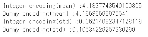
ジャンルデータを含めると、整数モデルとダミーエンコードされた線形モデルの平均にわずかな違いが見られます。ダミーエンコードされたモデルの標準は、整数エンコードされたモデルよりもまだ高いです。
次はSVRモデルです。
 #Excluding  genres
from sklearn import svm #整数エンコーディング

X = df.drop(labels = ['Category','Rating','Genres','Genres_c'],axis = 1)
y = df.Rating
X_train, X_test, y_train, y_test = train_test_split(X, y, test_size=0.30)

model2 = svm.SVR()
model2.fit(X_train,y_train)

Results2 = model2.predict(X_test)

resultsdf = resultsdf.append(Evaluationmatrix_dict(y_test,Results2, name = 'SVM - Integer'),ignore_index = True)
 #dummy  based


X_d = df2.drop(labels = ['Rating','Genres','Category_c','Genres_c'],axis = 1)
y_d = df2.Rating

X_train_d, X_test_d, y_train_d, y_test_d = train_test_split(X_d, y_d, test_size=0.30)

model2 = svm.SVR()
model2.fit(X_train_d,y_train_d)

Results2_d = model2.predict(X_test_d)

resultsdf = resultsdf.append(Evaluationmatrix_dict(y_test_d,Results2_d, name = 'SVM - Dummy'),ignore_index = True)plt.figure(figsize=(12,7))
sns.regplot(x=Results2,y=y_test,color='teal', label = 'Integer', marker = 'x')
sns.regplot(x=Results2_d,y=y_test_d,color='orange',label = 'Dummy')
plt.legend()
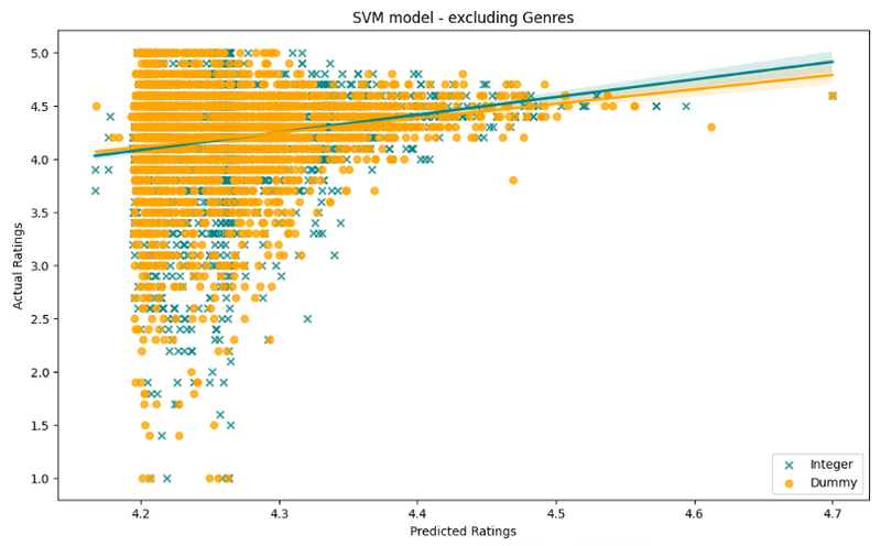
plt.title('SVM model - excluding Genres')
plt.xlabel('Predicted Ratings')
plt.ylabel('Actual Ratings')
plt.show()出力
print ('Integer encoding(mean) :' + str(Results2.mean()))
print ('Dummy encoding(mean) :'+ str(Results2_d.mean()))
print ('Integer encoding(std) :' + str(Results2.std()))
print ('Dummy encoding(std) :'+ str(Results2_d.std()))
出力
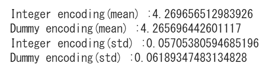
全体として、モデルは、実際の評価がそうではなかったにもかかわらず、かなりの評価が約4.2になると予測しました。散布図を見ると、整数エンコードされたモデルは、このインスタンスでよりよく浸透しているようです。
これまでと同様にダミーエンコードモデルは、整数エンコードモデルよりも高い標準を持っています。
 #Integer  encoding, including Genres_c
model2a = svm.SVR()

X = df.drop(labels = ['Category','Rating','Genres'],axis = 1)
y = df.Rating

X_train, X_test, y_train, y_test = train_test_split(X, y, test_size=0.30)

model2a.fit(X_train,y_train)

Results2a = model2a.predict(X_test)
 #評価
resultsdf = resultsdf.append(Evaluationmatrix_dict(y_test,Results2a, name = 'SVM(inc Genres) - Integer'),ignore_index = True)
 #dummy  encoding, including Genres_c
model2a = svm.SVR()

X_d = df2.drop(labels = ['Rating','Genres','Category_c'],axis = 1)
y_d = df2.Rating

X_train_d, X_test_d, y_train_d, y_test_d = train_test_split(X_d, y_d, test_size=0.30)

model2a.fit(X_train_d,y_train_d)

Results2a_d = model2a.predict(X_test_d)
 #評価
resultsdf = resultsdf.append(Evaluationmatrix_dict(y_test_d,Results2a_d, name = 'SVM(inc Genres) - Dummy'),ignore_index = True)plt.figure(figsize=(12,7))
sns.regplot(x=Results2a,y=y_test,color='teal', label = 'Integer', marker = 'x')
sns.regplot(x=Results2a_d,y=y_test_d,color='orange',label = 'Dummy')
plt.legend()
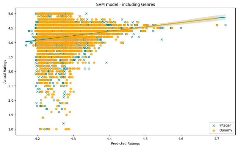
plt.title('SVM model - including Genres')
plt.xlabel('Predicted Ratings')
plt.ylabel('Actual Ratings')
plt.show()出力
print ('Integer encoding(mean) :' + str(Results2a.mean()))
print ('Dummy encoding(mean) :'+ str(Results2a_d.mean()))
print ('Integer encoding(std) :' + str(Results2a.std()))
print ('Dummy encoding(std) :'+ str(Results2a_d.std()))
出力
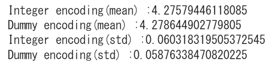
ジャンルデータを含めると、実際の結果と予測結果を比較する回帰線が整数エンコードモデルのそれと非常に似ているため、ダミーエンコーディングモデルはより良いパフォーマンスを発揮しているようです。
さらにダミーエンコードモデルの標準は大幅に低下し、整数エンコードモデルと比較して平均が高くなっています。
次はランダムフォレスト回帰モデルです。
from sklearn.ensemble import RandomForestRegressor
 #整数エンコーディング
X = df.drop(labels = ['Category','Rating','Genres','Genres_c'],axis = 1)
y = df.Rating
X_train, X_test, y_train, y_test = train_test_split(X, y, test_size=0.30)
model3 = RandomForestRegressor()
model3.fit(X_train,y_train)
Results3 = model3.predict(X_test)
 #評価
resultsdf = resultsdf.append(Evaluationmatrix_dict(y_test,Results3, name = 'RFR - Integer'),ignore_index = True)
 #ダミーエンコーディング

X_d = df2.drop(labels = ['Rating','Genres','Category_c','Genres_c'],axis = 1)
y_d = df2.Rating
X_train_d, X_test_d, y_train_d, y_test_d = train_test_split(X_d, y_d, test_size=0.30)
model3_d = RandomForestRegressor()
model3_d.fit(X_train_d,y_train_d)
Results3_d = model3_d.predict(X_test_d)
 #評価
resultsdf = resultsdf.append(Evaluationmatrix_dict(y_test,Results3_d, name = 'RFR - Dummy'),ignore_index = True)plt.figure(figsize=(12,7))
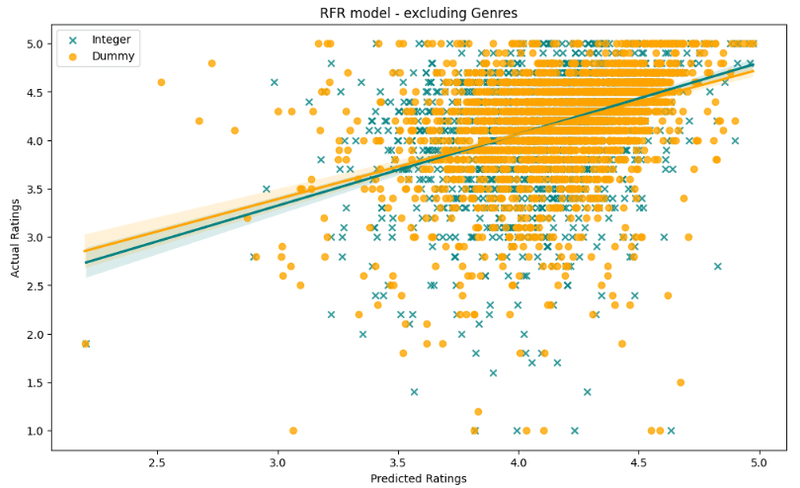
sns.regplot(x=Results3,y=y_test,color='teal', label = 'Integer', marker = 'x')
sns.regplot(x=Results3_d,y=y_test_d,color='orange',label = 'Dummy')
plt.legend()
plt.title('RFR model - excluding Genres')
plt.xlabel('Predicted Ratings')
plt.ylabel('Actual Ratings')
plt.show()出力
print ('Integer encoding(mean) :' + str(Results3.mean()))
print ('Dummy encoding(mean) :'+ str(Results3_d.mean()))
print ('Integer encoding(std) :' + str(Results3.std()))
print ('Dummy encoding(std) :'+ str(Results3_d.std()))
出力
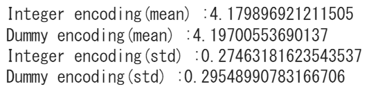
一見するとランダムフォレストモデルはプロットされた散布図を見るだけで、最高の予測結果を出したと言えるでしょう。全体として、整数とダミーエンコードモデルの両方のモデルは、ダミーエンコードされたモデルの方が全体的な予測平均が高くなりますが、比較的類似したパフォーマンスを発揮するようです。
 #for  integer
Feat_impt = {}
for col,feat in zip(X.columns,model3.feature_importances_):
    Feat_impt[col] = feat

Feat_impt_df = pd.DataFrame.from_dict(Feat_impt,orient = 'index')
Feat_impt_df.sort_values(by = 0, inplace = True)
Feat_impt_df.rename(index = str, columns = {0:'Pct'},inplace = True)

plt.figure(figsize= (14,10))
Feat_impt_df.plot(kind = 'barh',figsize= (14,10),legend = False)
plt.sho出力
出力
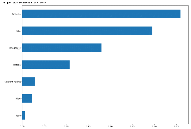
評価に影響を与えるものを見ると、トップ4はレビュー、サイズ、カテゴリ、インストール数が最も影響力があるようです。
 #for  dummy
Feat_impt_d = {}
for col,feat in zip(X_d.columns,model3_d.feature_importances_):
    Feat_impt_d[col] = feat

Feat_impt_df_d = pd.DataFrame.from_dict(Feat_impt_d,orient = 'index')
Feat_impt_df_d.sort_values(by = 0, inplace = True)
Feat_impt_df_d.rename(index = str, columns = {0:'Pct'},inplace = True)

plt.figure(figsize= (14,10))
Feat_impt_df_d.plot(kind = 'barh',figsize= (14,10),legend = False)
plt.show()
出力
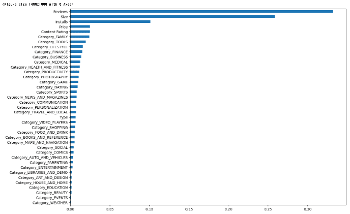
内訳をさらに見ると、確かにレビュー、サイズ、インストール数は、アプリの評価の予測性に大きな影響を与えているようです。アプリのツールカテゴリが、食べ物や飲み物のカテゴリと比較して、非常に高いレベルの予測性を持っていることがうかがえます。
 #Including  Genres_C
 #整数エンコーディング
X = df.drop(labels = ['Category','Rating','Genres'],axis = 1)
y = df.Rating
X_train, X_test, y_train, y_test = train_test_split(X, y, test_size=0.30)
model3a = RandomForestRegressor()
model3a.fit(X_train,y_train)
Results3a = model3a.predict(X_test)
 #評価
resultsdf = resultsdf.append(Evaluationmatrix_dict(y_test,Results3a, name = 'RFR(inc Genres) - Integer'),ignore_index = True)
 #ダミーエンコーディング

X_d = df2.drop(labels = ['Rating','Genres','Category_c'],axis = 1)
y_d = df2.Rating
X_train_d, X_test_d, y_train_d, y_test_d = train_test_split(X_d, y_d, test_size=0.30)
model3a_d = RandomForestRegressor()
model3a_d.fit(X_train_d,y_train_d)
Results3a_d = model3a_d.predict(X_test_d)
 #評価
resultsdf = resultsdf.append(Evaluationmatrix_dict(y_test,Results3a_d, name = 'RFR(inc Genres) - Dummy'),ignore_index = True)plt.figure(figsize=(12,7))
sns.regplot(x=Results3a,y=y_test,color='teal', label = 'Integer', marker = 'x')
sns.regplot(x=Results3a_d,y=y_test_d,color='orange',label = 'Dummy')
plt.legend()
plt.title('RFR model - including Genres')
plt.xlabel('Predicted Ratings')
plt.ylabel('Actual Ratings')
plt.show()出力
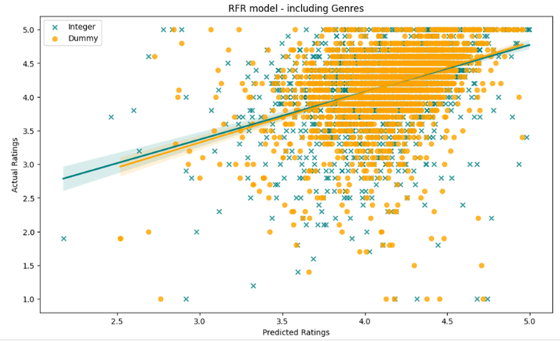
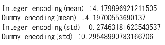
print ('Integer encoding(mean) :' + str(Results3.mean()))
print ('Dummy encoding(mean) :'+ str(Results3_d.mean()))
print ('Integer encoding(std) :' + str(Results3.std()))
print ('Dummy encoding(std) :'+ str(Results3_d.std()))
出力
 #for  integer
Feat_impt = {}
for col,feat in zip(X.columns,model3a.feature_importances_):
    Feat_impt[col] = feat

Feat_impt_df = pd.DataFrame.from_dict(Feat_impt,orient = 'index')
Feat_impt_df.sort_values(by = 0, inplace = True)
Feat_impt_df.rename(index = str, columns = {0:'Pct'},inplace = True)

plt.figure(figsize= (14,10))
Feat_impt_df.plot(kind = 'barh',figsize= (14,10),legend = False)
plt.show()
出力
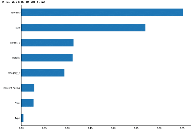
この結果から、ジャンルセクションは決定木の作成において実際に重要な役割を果たしているように思われます。しかし、それを除外しても、結果に大きな影響を与えるようには見えません。
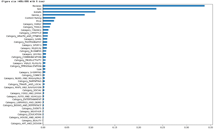
 #for  dummy
Feat_impt_d = {}
for col,feat in zip(X_d.columns,model3a_d.feature_importances_):
    Feat_impt_d[col] = feat

Feat_impt_df_d = pd.DataFrame.from_dict(Feat_impt_d,orient = 'index')
Feat_impt_df_d.sort_values(by = 0, inplace = True)
Feat_impt_df_d.rename(index = str, columns = {0:'Pct'},inplace = True)

plt.figure(figsize= (14,10))
Feat_impt_df_d.plot(kind = 'barh',figsize= (14,10),legend = False)
plt.show()
出力
resultsdf.set_index('Series Name', inplace = True)

plt.figure(figsize = (10,12))
plt.subplot(3,1,1)
resultsdf['Mean Squared Error'].sort_values(ascending = False).plot(kind = 'barh',color=(0.3, 0.4, 0.6, 1), title = 'Mean Squared Error')
plt.subplot(3,1,2)
resultsdf['Mean Absolute Error'].sort_values(ascending = False).plot(kind = 'barh',color=(0.5, 0.4, 0.6, 1), title = 'Mean Absolute Error')
plt.subplot(3,1,3)
resultsdf['Mean Squared Log Error'].sort_values(ascending = False).plot(kind = 'barh',color=(0.7, 0.4, 0.6, 1), title = 'Mean Squared Log Error')
plt.show()
出力
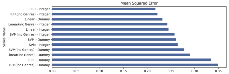
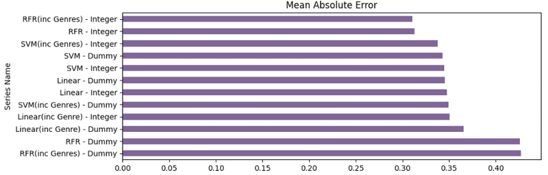
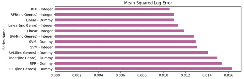
最後に、結果を見ると、どのモデルが最高の予測精度と最も低い誤差項を持っているかを見下すのは簡単ではありません。このラウンドのデータを基礎として、ジャンルを含むダミーエンコードされたSVMモデルは、全体的なエラー率が最も低く、遺伝子を含む整数エンコードされたRFRモデルが続きます。しかし、すべてのモデルはエラー項の点で非常に近いように見えるので、この結果は変わる可能性があります。
まとめ
私にとって非常に驚くべきことは、表面上はRFR整数モデルと非常によく似たように動作しているように見えたにもかかわらず、RFRダミーモデルが他のモデルと比較してエラー項が大幅に多いことです。
この記事が気に入ったらサポートをしてみませんか?