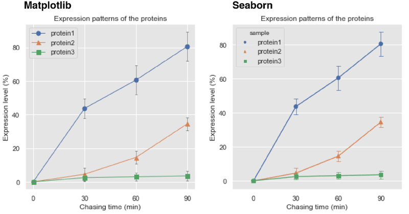
細胞内に発現する3つのタンパク質の相対量変化を例にした折れ線グラフの描画 (Matplotlib, Seaborn)

3種類のタンパク質 Protein1, Protein2, Protein3について,あるタイムポイント(0分)から始めて90分まで,30分おきに細胞内発現量を経時的に定量・算出したデータを想定して,折れ線グラフを作成する方法を書き留める。
全てのデータは独立した三回の実験(exp_number:1-3)によって算出されたものと想定し,平均値をプロットし,エラーバーは標準偏差値を基に描く。
plotはMatplotlibの"ax.plot",とSeabornの"sns.pointplot"を利用する。
仮想データの準備
# import modules
import numpy as np
import random
import pandas as pd
import matplotlib.pyplot as plt
import seaborn as sns
sns.set_style('darkgrid',{"axes.facecolor": ".9"})

# Data preparation
# 0min
a,e,i= list([0]*3),list([0]*3),list([0]*3)

# 30 min
np.random.seed(42)
b = [np.random.uniform(30,50) for i in range (1,4)]
f = [np.random.uniform(0,15) for i in range (1,4)]
j = [np.random.uniform(0,5) for i in range (1,4)]

# 60 min
np.random.seed(42)
c = [np.random.uniform(40,70) for i in range (1,4)]
g = [np.random.uniform(10,25) for i in range (1,4)]
k = [np.random.uniform(0,6) for i in range (1,4)]

# 90 min
np.random.seed(42)
d = [np.random.uniform(60,90) for i in range (1,4)]
h = [np.random.uniform(30,45) for i in range (1,4)]
l = [np.random.uniform(0,7) for i in range (1,4)]

#protein1
protein1 =pd.DataFrame({'0':a, 30:b, 60:c, 90:d})
protein1['sample'] = ['protein1']*3
protein1['exp_number']= [1,2,3]
protein1 =protein1.iloc[:,[4,5,0,1,2,3]]

#protein2
protein2 =pd.DataFrame({'0':e, 30:f, 60:g, 90:h})
protein2['sample'] = ['protein2']*3
protein2['exp_number']= [1,2,3]
protein2 = protein2.iloc[:,[4,5,0,1,2,3]]

#protein3
protein3 =pd.DataFrame({'0':i, 30:j, 60:k, 90:l})
protein3['sample'] = ['protein3']*3
protein3['exp_number']= [1,2,3]
protein3 = protein3.iloc[:,[4,5,0,1,2,3]]

print('protein1:')
display(protein1)
print('protein2:')
display(protein2)
print('protein3:')
display(protein3)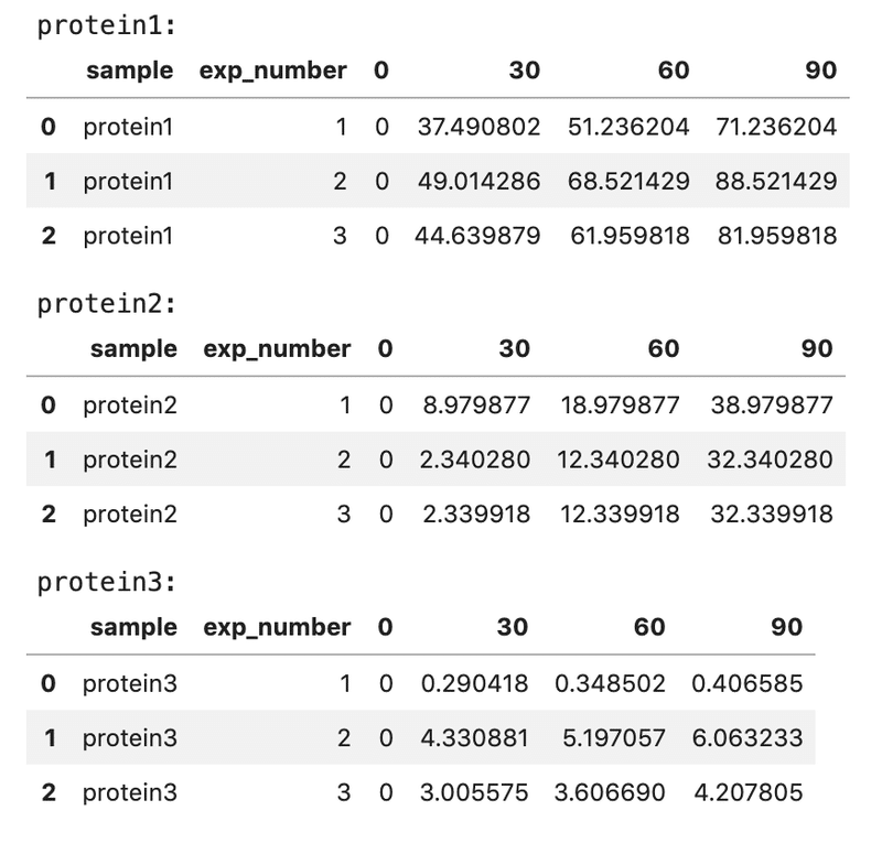
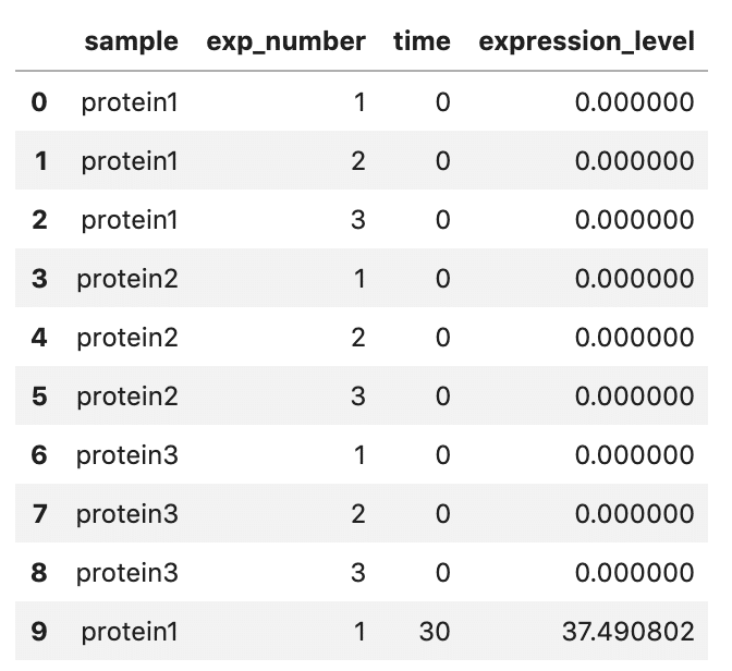
sns.pointplotで描画するためにデータをpd.meltで'tidy'に
protein1-3のデータを縦に連結(concat)
df = pd.concat([protein1,protein2,protein3], axis = 0 , ignore_index=True)
display(df)
meltする
df_melt = pd.melt(df, id_vars=['sample', 'exp_number'],
                 var_name='time', value_name='expression_level')
df_melt.head(10)
・id_vars :そのまま残す変数: 'sample', exp_number
・var_name : meltするvariant('0', '30', '60', '90')につける名前を指定: 'time'
・value_name : meltするvalues(数値)につける名前を指定: 'expression_level'
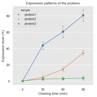
sns.lineplotで描画
fig,ax = plt.subplots(figsize = (5,5))
sns.set()
sns.set_style('darkgrid',{"axes.facecolor": ".9"})

ax =sns.pointplot(x='time', y = 'expression_level', hue = 'sample',
                kind='point',
                data = df_melt,
                markers = ['o','^','s'],
                style = 'sample', scale = .5, ci = 'sd', capsize=.1, errwidth=.75)
# sns.pointplotではmarker size とlinewidthが別々に指定できない
# -> 下記 plt.setp()でmarkersizeを指定する

ax.set(ylabel = 'Expression level (%)', xlabel = 'Chasing time (min)', title = 'Expression patterns of the proteins')
plt.setp(ax.collections, sizes = [40]);  # markersizeをlinewidthと独立に指定する
(ポイント)コード最終行のように,markersize を変えたい時は
plt.setp(ax.collections, sizes = [40]);
で markersizeを指定する
エラーバーの色を黒くしたかったんだけど出来ずに断念(´・ω・`) 変える方法はあるのだろうか???
ax.plotで描画するためにmeanとsdを算出
(流れ)
(1)'sample'と'time'でgroupby してmeanとsdを算出。
(2)その後,meanとsdそれぞれについてpivotでindexを'time'に, columnを'sample'に指定する。
(3)最後にmeanとsdのデータを横につなげる。
# Caluculate mean and modify dataframe
# mean
df_mean = df_melt.groupby(['sample','time',], as_index=False)['expression_level'].agg({'':[np.mean]})
df_mean = df_mean.pivot(index = 'time', columns='sample').iloc[[3,0,1,2],:].reset_index()
# sd
df_sd =df_melt.groupby(['sample','time',], as_index=False)['expression_level'].agg({'':[np.std]})
df_sd = df_sd.pivot(index = 'time', columns='sample').iloc[[3,0,1,2],:].reset_index()

print('mean:')
display(df_mean)
print('sd:')
display(df_sd)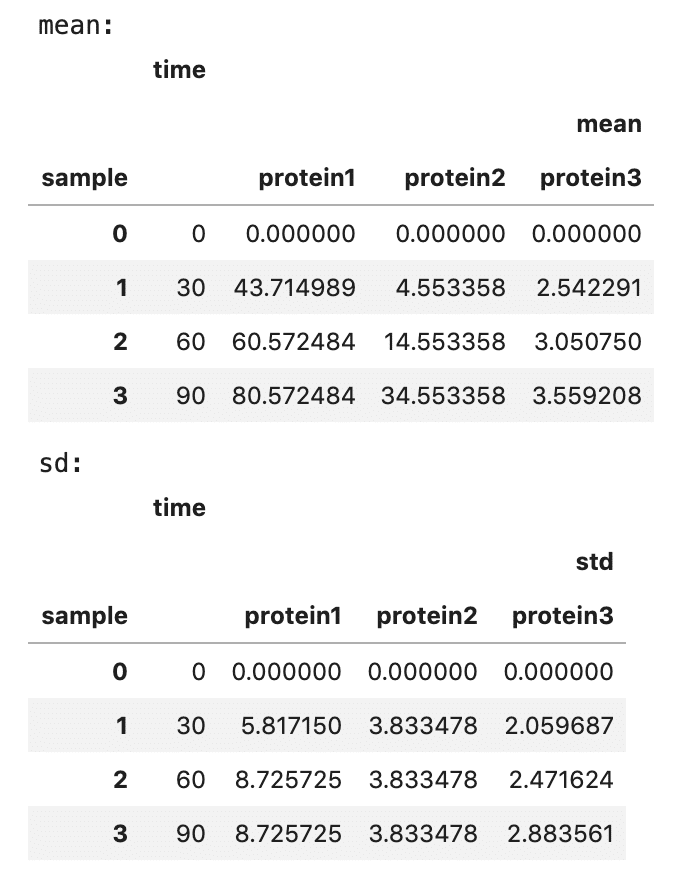
# mead と sd のデータを連結
df_meansd = pd.merge(df_mean, df_sd, on = 'time')
df_meansd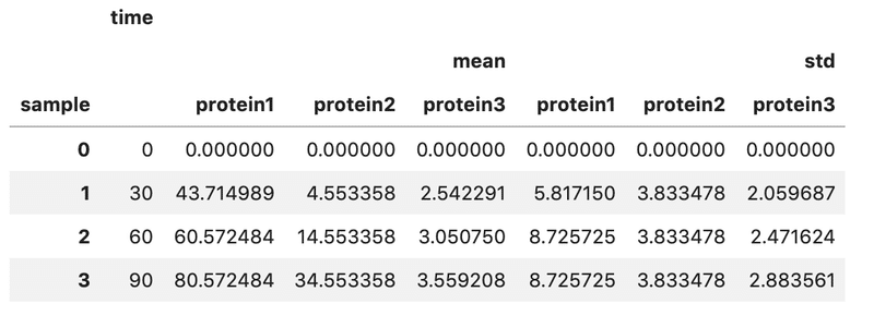
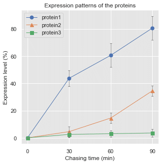
ax.plotでグラフ描画
multi columでは列の指定が普段と異なる。 例えばdf_meansd中のmeanのprotein1 を指定する場合は:
df_meansd['', 'mean', 'protein1']と上から順にカラム名を指定する。
fig,ax = plt.subplots(figsize = (5,5))

# Parameters
sample_name = ["protein"+str(i) for i in range(1,4)]
marker = ['o','^','s']

for m,col in zip(marker, sample_name):
    ax.plot([0,30,60,90], df_meansd['', 'mean', col],
            marker = m, markersize=7, linewidth =1 , label = col)

    ax.errorbar([0,30,60,90], df_meansd['', 'mean', col], df_meansd['', 'std', col],
                linestyle='', color='gray', linewidth =.75, capsize=2, label = '')
    # label= ''にしないとエラーバーの凡例が入ってしまう

    from matplotlib import ticker
ax.xaxis.set_major_locator(ticker.MultipleLocator(30)) # xtick を30min区切りに

ax.set(ylabel = 'Expression level (%)', xlabel = 'Chasing time (min)', title = 'Expression patterns of the proteins')
ax.legend()
おしまい。
この記事が気に入ったらサポートをしてみませんか?