パンシャープン処理とは

近年のリモートセンシングデータは、パンクロマティックセンサーによって高解像度のモノクロ画像（＝パンクロマティック画像）を取得できます。一方、解像度は少し劣るものの、マルチスペクトルセンサーからはカラー情報が得られるため、この両者の特性を擬似的に合成させることにより、高解像度カラー画像の作成が可能となります。この方法がパンシャープン処理です。
※合成させるデータ間の空間分解能の差は2倍〜4倍程度が適当とされている。

今回はLandsat 8のBand2~5（空間分解能：30m）とBand8（空間分解能：15m）がすでに手元にある前提で進めていきます。
ちなみに、下記記事の続きになるので、よかったらこちらも見てみてください。Google Earth EngineとGDALでさくっとパンシャープン処理（HSV変換とBrovey変換）を適用させてみました。

パンシャープン処理の手法

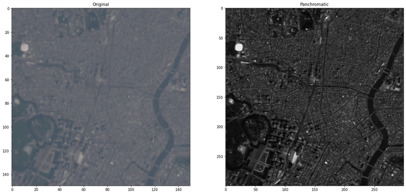
本記事で扱う4バンド＋モノクロ画像を読み込んでみましょう。

import numpy as np
import xarray as xr
import matplotlib.pyplot as plt

import skimage.color as color
from skimage.transform import rescale

blue = xr.open_rasterio(f'B2_20200429.tif').values[0]
green = xr.open_rasterio(f'B3_20200429.tif').values[0]
red = xr.open_rasterio(f'B4_20200429.tif').values[0]
ni = xr.open_rasterio(f'B5_20200429.tif').values[0]
pan = xr.open_rasterio(f'B8_20200429.tif').values[0]

def convert(band, gamma):
    band = np.clip(band, 0, 1)
    band = np.power(band, 1/gamma)
    return band

x_min = 250; x_max = 400; y_min = 250; y_max = 400

plt.figure(figsize=(20,20))

plt.subplot(1,2,1)
plt.imshow(np.dstack([convert(red, 2.2)[y_min:y_max, x_min:x_max], convert(green, 2.2)[y_min:y_max, x_min:x_max], convert(blue, 2.2)[y_min:y_max, x_min:x_max]]), vmax=0.4)
plt.title('Original')

plt.subplot(1,2,2)
plt.imshow(pan[y_min*2:y_max*2, x_min*2:x_max*2], cmap=plt.get_cmap('gray'), vmax=0.4)
plt.title('Panchromatic')

このサイトに載っている計算式や論文を参考にしつつ、パンシャープン処理のコード書いていきます。

その前に、下準備としてマルチスペクトル画像（B2, B3, B4, B5）をパンクロマティック画像（B8）のサイズに合わせる必要があります。

ysize, xsize = red.shape # (748, 613)

rgbn = np.empty((4, ysize, xsize))
rgbn[0,:,:] = red
rgbn[1,:,:] = green
rgbn[2,:,:] = blue
rgbn[3,:,:] = ni

rgbn_rescaled = np.empty((4, ysize*2, xsize*2)) # (1496, 1226)
for i in range(4):
    rgbn_rescaled[i,:,:] = rescale(rgbn[i,:,:], (2,2))
    
# 画像間の演算処理を行うために、パンクロマティック画像のサイズ（1495, 1226）に合わせる
rgbn_rescaled = rgbn_rescaled[:,:pan.shape[0],:]

# オリジナルとパンシャープン画像の描画
def draw(r_pan, g_pan, b_pan, method=None):
    x_min = 250; x_max = 400; y_min = 250; y_max = 400

    plt.figure(figsize=(20,20))

    plt.subplot(1,2,1)
    plt.imshow(np.dstack([convert(red, 2.2)[y_min:y_max, x_min:x_max], convert(green, 2.2)[y_min:y_max, x_min:x_max], convert(blue, 2.2)[y_min:y_max, x_min:x_max]]), vmax=0.4)
    plt.title('Original')

    plt.subplot(1,2,2)
    plt.imshow(np.dstack([r_pan[y_min*2:y_max*2, x_min*2:x_max*2], g_pan[y_min*2:y_max*2, x_min*2:x_max*2], b_pan[y_min*2:y_max*2, x_min*2:x_max*2]]))
    plt.title(f'method={method}')
    
    
R = rgbn_rescaled[0,:,:]
G = rgbn_rescaled[1,:,:]
B = rgbn_rescaled[2,:,:]
NIR = rgbn_rescaled[3,:,:]

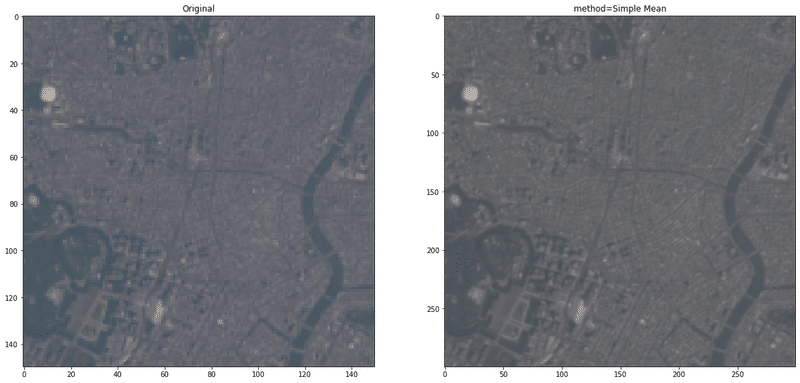
Simple Mean

r_pan = convert(0.5 * (R+ pan), 2.2)
g_pan = convert(0.5 * (G + pan), 2.2)
b_pan = convert(0.5 * (B + pan), 2.2)

draw(r_pan, g_pan, b_pan, method='Simple Mean')

Esri

ADJ = pan-rgbn_rescaled.mean(axis=0)

r_pan = convert((R + ADJ), 2.2)
g_pan = convert((G + ADJ), 2.2)
b_pan = convert((B + ADJ), 2.2)

draw(r_pan, g_pan, b_pan, method='Esri')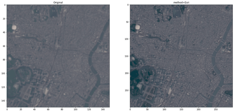

Brovey

W = 0.2
DNF = (pan - W*NIR)/(W*R+W*G+W*B)

r_pan = convert((R * DNF), 2.2)
g_pan = convert((G * DNF), 2.2)
b_pan = convert((B * DNF), 2.2)

draw(r_pan, g_pan, b_pan, method='Brovey')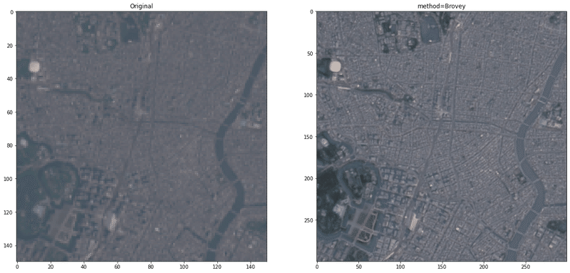

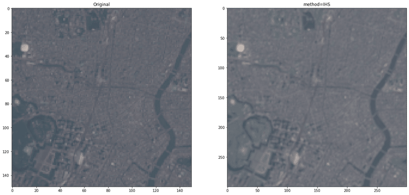
IHS

W = 0.2
I = pan - NIR*W

r_pan = convert(R+(pan-I), 2.2)
g_pan = convert(G+(pan-I), 2.2)
b_pan = convert(B+(pan-I), 2.2)

draw(r_pan, g_pan, b_pan, method='IHS')

なんか画質粗い、、、

Fast-IHS

従来のIHSによるパンシャープン処理のアップデート版？画質やスペクトルの歪みが改善されたとのこと。（https://www.researchgate.net/publication/259745690_Application_of_IHS_Pan-Sharpening_techniques_to_IKONOS_images）

a = 0.75; b = 0.25
I = ( R + a*G + b*B + NIR ) / 3.0

r_pan = convert(R+(pan-I), 2.2)
g_pan = convert(G+(pan-I), 2.2)
b_pan = convert(B+(pan-I), 2.2)

draw(r_pan, g_pan, b_pan, method='Fast-IHS')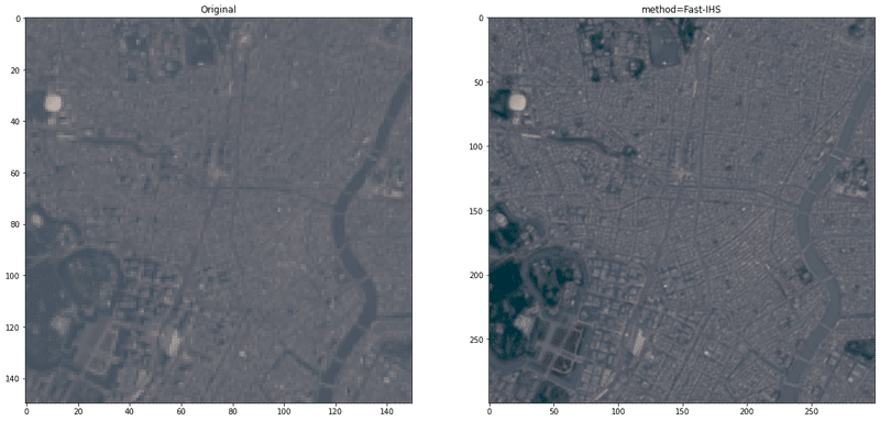

主成分分析法

衛星画像の複数バンドに対して、主成分分析（PCA; principal component analysis）を適用後の第一主成分は、その画像の強度成分にほぼ等しいことがわかっているので、IHS変換と同じ要領で、「第一主成分≒パンクロマティック画像」とみなし、両者を入れ替えて、逆主成分分析を行う。
IHS変換は3バンドという制限がある一方で、主成分分析法では元のマルチスペクトル画像のバンド数にかかわらず、パンシャープン処理が可能である。

逆主成分分析を適用させる前の重要な前処理として、パンクロマティック画像のDN値分布と第一主成分の分布を合わせるためのヒストグラムマッチングというものがあるらしいです。（https://www.mdpi.com/2072-4292/8/10/794）

from sklearn.decomposition import PCA

rgbnir = np.dstack([R, G, B, NIR])

rgbnir_reshape = rgbnir.reshape(rgbnir.shape[0]*rgbnir.shape[1], rgbnir.shape[2])
pan_reshape = pan.reshape(rgbnir.shape[0]*rgbnir.shape[1])


def hist_matching(pan_reshape, rgbnir_components):   
    source_shape = pan_reshape.shape
    source = pan_reshape.ravel()
    template = rgbnir_components[:, 0].ravel()
    
    s_values, bin_idx, s_counts = np.unique(source, return_inverse=True, return_counts=True)
    t_values, t_counts = np.unique(template, return_counts=True)
    
    s_quantiles = np.cumsum(s_counts).astype(np.float64)
    s_quantiles /= s_quantiles[-1]
    
    t_quantiles = np.cumsum(t_counts).astype(np.float64)
    t_quantiles /= t_quantiles[-1]

    return np.interp(s_quantiles, t_quantiles, t_values)[bin_idx].reshape(source_shape)


pca = PCA(4)
rgbnir_components = pca.fit_transform(rgbnir_reshape)
rgbnir_components[:, 0] = hist_matching(pan_reshape, rgbnir_components)
rgbnir_components = pca.inverse_transform(rgbnir_components)
rgbnir_components = rgbnir_components.reshape(rgbnir.shape[0], rgbnir.shape[1], rgbnir.shape[2])

r_pan = convert(rgbnir_components[:, :, 0], 2.2)
g_pan = convert(rgbnir_components[:, :, 1], 2.2)
b_pan = convert(rgbnir_components[:, :, 2], 2.2)

draw(r_pan, g_pan, b_pan, method='PCA')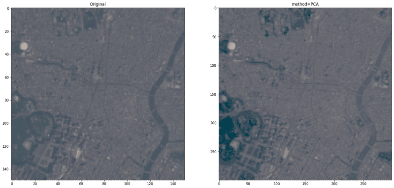

複数バンドデータの空間情報を生かした主成分分析と似た手法として、Wavelet変換もあります。
Wavelet変換はスペクトル解析の一つで、色の空間的分布を局所的に、解像度を変えることができる手法です。マルチスペクトル画像の各バンドとパンクロマティック画像それぞれにWavelet変換を施し、パンクロマティック画像の低い空間スペクトル部分のWavelet係数を、マルチスペクトル画像の低い空間スペクトルに入れ替え、パンクロマティック画像のWavelet逆変換を行うことで、パンシャープン画像が完成するはず。