ChatGPTにIsolation Forestの異常値判定を教えてもらったメモ。特に多次元データセットでの異常値判定は便利なので、特徴量生成に生かしたい。

Isolation Forestとは：多次元データでの異常値検出

Isolation Forestは異常値検出に特化した機械学習アルゴリズムで、特に多次元データセットでその能力を発揮します。ランダム分割を利用してデータポイントを孤立させ、異常値を効率的に識別します。

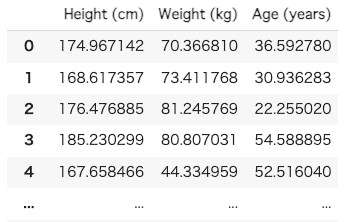
サンプルデータの生成：身長、体重、年齢

身長、体重、年齢のサンプルデータをランダム生成し、Isolation Forestの実践的な適用を探ります。

異常値判定の例

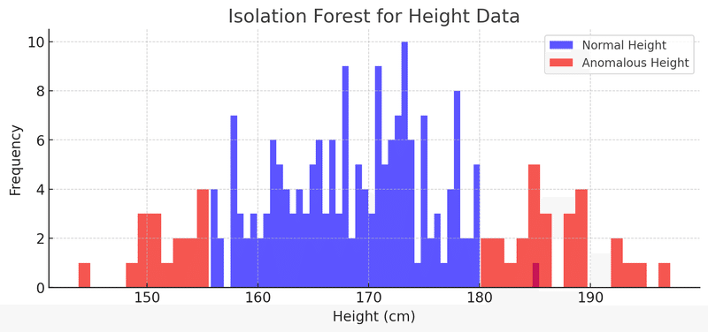
1次元での異常値判定：身長データの分析

1次元データセットでは、身長データに対してIsolation Forestを適用し、異常値を識別します。このシンプルな例が、アルゴリズムの効果を示しています。

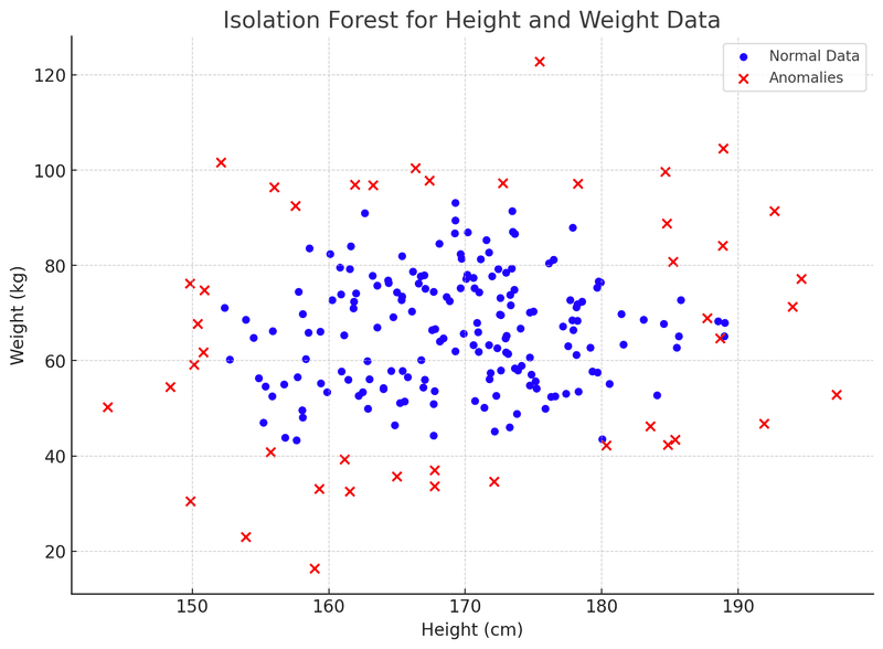
2次元での異常値判定：身長と体重の関係

2次元データセットでは、身長と体重の組み合わせに焦点を当て、異常値の特定を行います。このアプローチは、特徴量の相互作用を考慮に入れます。

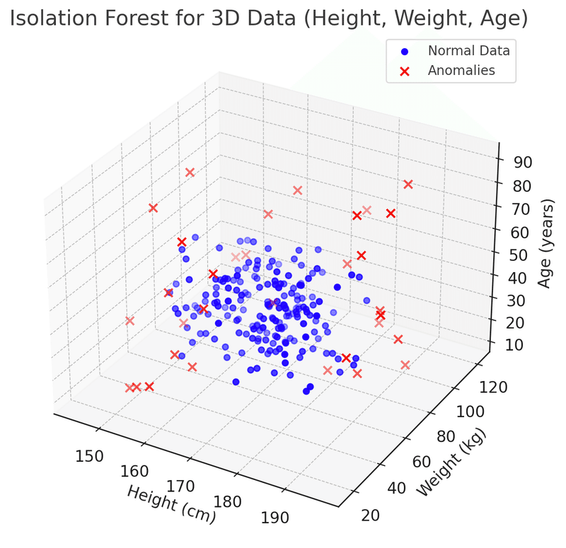
3次元での異常値判定：包括的な分析

身長、体重、年齢を含む3次元データにおいて、Isolation Forestは複数の特徴量を組み合わせて異常値を特定します。この複合的な分析がアルゴリズムの強みです。 

コード

サンプルデータ生成

import numpy as np
import pandas as pd

# パラメータ設定
height_mean = 170  # 身長の平均値 (cm)
height_std = 10    # 身長の標準偏差 (cm)
weight_mean = 65   # 体重の平均値 (kg)
weight_std = 15    # 体重の標準偏差 (kg)
age_min = 20       # 年齢の最小値 (歳)
age_max = 60       # 年齢の最大値 (歳)

np.random.seed(42)  # 再現性のための乱数シード
normal_height = np.random.normal(height_mean, height_std, 200)
normal_weight = np.random.normal(weight_mean, weight_std, 200)
normal_age = np.random.uniform(age_min, age_max, 200)
X_normal = np.stack((normal_height, normal_weight, normal_age), axis=1)

anomaly_height = np.random.uniform(height_mean - 3*height_std, height_mean + 3*height_std, 20)
anomaly_weight = np.random.uniform(weight_mean - 3*weight_std, weight_mean + 3*weight_std, 20)
anomaly_age = np.random.uniform(0, 100, 20)  # 通常の範囲外の年齢
X_anomalies = np.stack((anomaly_height, anomaly_weight, anomaly_age), axis=1)

# 正常値と異常値が混ざったデータセットの作成
all_data = np.vstack((X_normal, X_anomalies))

# データフレームの作成
df_mixed = pd.DataFrame(all_data, columns=['Height (cm)', 'Weight (kg)', 'Age (years)'])

１次元データ（身長）

import matplotlib.pyplot as plt
from sklearn.ensemble import IsolationForest

clf_height = IsolationForest(random_state=42)
height_data = df_mixed['Height (cm)'].values.reshape(-1, 1)
clf_height.fit(height_data)
y_pred_height = clf_height.predict(height_data)

plt.figure(figsize=(10, 4))
plt.hist(height_data[y_pred_height == 1], bins=50, alpha=0.7, label='Normal Height', color='blue')
plt.hist(height_data[y_pred_height == -1], bins=50, alpha=0.7, label='Anomalous Height', color='red')
plt.legend()
plt.title("Isolation Forest for Height Data")
plt.xlabel('Height (cm)')
plt.ylabel('Frequency')
plt.show()

２次元データ（身長、体重）

clf_height_weight = IsolationForest(random_state=42)
height_weight_data = df_mixed[['Height (cm)', 'Weight (kg)']].values
clf_height_weight.fit(height_weight_data)
y_pred_height_weight = clf_height_weight.predict(height_weight_data)

plt.figure(figsize=(10, 7))
plt.scatter(height_weight_data[y_pred_height_weight == 1, 0], height_weight_data[y_pred_height_weight == 1, 1], c='blue', marker='o', s=20, label='Normal Data')
plt.scatter(height_weight_data[y_pred_height_weight == -1, 0], height_weight_data[y_pred_height_weight == -1, 1], c='red', marker='x', s=40, label='Anomalies')
plt.legend()
plt.title("Isolation Forest for Height and Weight Data")
plt.xlabel('Height (cm)')
plt.ylabel('Weight (kg)')
plt.show()

３次元データ（身長、体重、年齢）

from mpl_toolkits.mplot3d import Axes3D

clf_3d = IsolationForest(random_state=42)
three_dim_data = df_mixed[['Height (cm)', 'Weight (kg)', 'Age (years)']].values
clf_3d.fit(three_dim_data)
y_pred_3d = clf_3d.predict(three_dim_data)

# 3次元データ（身長、体重、年齢）の異常値検出と可視化
fig = plt.figure(figsize=(10, 7))
ax_3d = fig.add_subplot(111, projection='3d')
ax_3d.scatter(three_dim_data[y_pred_3d == 1, 0], three_dim_data[y_pred_3d == 1, 1], three_dim_data[y_pred_3d == 1, 2], c='blue', marker='o', s=20, label='Normal Data')
ax_3d.scatter(three_dim_data[y_pred_3d == -1, 0], three_dim_data[y_pred_3d == -1, 1], three_dim_data[y_pred_3d == -1, 2], c='red', marker='x', s=40, label='Anomalies')
ax_3d.legend()
ax_3d.set_title("Isolation Forest for 3D Data (Height, Weight, Age)")
ax_3d.set_xlabel('Height (cm)')
ax_3d.set_ylabel('Weight (kg)')
ax_3d.set_zlabel('Age (years)')
plt.show()