大学時代の制御工学の授業を思い出しながら、（私の勝手な主観判断で）必要最低限の知識を「虎の巻」として書いていこうと思います。こんな記事を書こうと思ったのは、実は最近になって「ちゃんと制御を考えるように！」と、とある大先生から宿題をもらったからです。私自身、モノづくりをするときには制御をもっとしっかり論理的に検討しなければならないと思いつつも、期限の都合でほどほどで切り上げていた過去の自分に反省し、現実の開発現場と学問域の制御をどうしたらつなげられるかを考えていきたいと思います。
そのためにも、まずは基本の「キ」となる部分を超最小限の内容で虎の巻としたいと思います。

ラプラス変換と伝達関数

簡単に言えば、次式の公式でラプラス変換をすると伝達関数が出てくるということです。

時間領域の式がラプラス変換によって周波数領域の式になるくらいしか大学当時は気にも留めませんでした。そして、伝達関数の方は、とりあえず大学の制御工学の授業で習うので、なんとなくシステムの表現なのかな？って感じてであまり深く考えずにいましたね。
この年になて、改めてラプラス変換をなんでするのかを考えてみると、大きかったり複雑なシステムをモデル化するのに便利なんだなと感じますし、ラプラス変換して伝達関数にすることでステップ応答やインパルス応答、各種周波数応答の計算がしやすかったりするメリットがあると感じますが、開発現場でどうしても大規模だったり複雑なシステムをモデル化したい、分析したいと思う機会が出てこないと、その価値を実感するのは難しいかもしれません。

Mapleでラプラス変換

それでは早速、Mapleで用意されているラプラス変換コマンドを使って、ラプラス変換をしてみましょう！ここで紹介する内容は記事の終わりに添付してあるMapleファイルにありますので、Mapleをお持ちの方は開きながら見ると理解しやすいと思います。

まず、初期化コマンドの「restart:」を記載します。
Mapleでコマンドを打っていく過程でメモリに意図しない変数がセットされていて意図しない結果になるのを防止するため、再実行後は初期化しますという意味の「restart:」を書いておきます。
そして、ラプラス変換のコマンド使うために「with(inttrans):」と記述しておきます。これでラプラス変換をコマンド1つで実行できます。

Mapleでのラプラス変換は、
「laplace(変換したい時間領域の関数, t, s)」というコマンドを使います。
１つ目の引数は「変換したい時間領域の関数」です。例えば「t」とか「t^2」とかです。「exp(t)」や「sin(t)」「cos(t)」でもよいです。
２つ目の引数は、１つめの引数の変数を指定します。通常は時間領域のため「t」とします。３つ目の引数はラプラス変換後の変数です。通常は「s」とします。
それでは、制御工学でよく使われるラプラス変換をMapleで計算してみましょう。

３つ目の「t^n」（tのn乗）はちょっと期待する形になりませんでしたが、それ以外は教科書に載っている形で変換されていますね。

今度は逆に、逆ラプラス変換をしてみましょう。
ラプラス変換のコマンドとほとんど同じです。
「invlaplace(変換したい周波数領域の関数, s, t)」というコマンドを使います。「inv」が前についているのと、２つ目の引数と３つ目の引数の「s」と「t」がラプラス変換のときと逆になっているだけですね。
ラプラス変換のときと同様に、制御工学でよく使われる逆ラプラス変換をMapleで計算してみましょう。

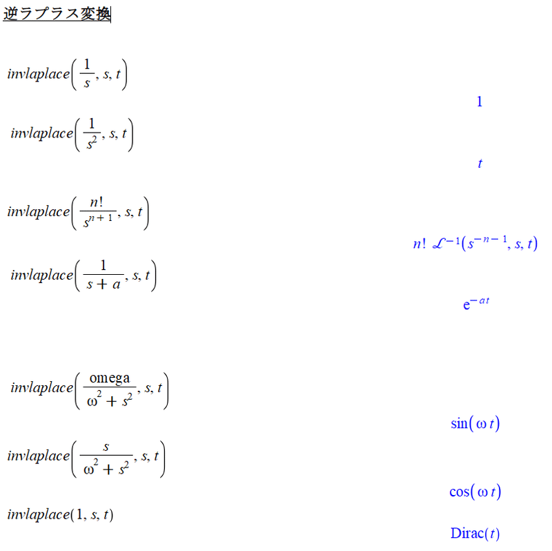
やはり、ラプラス変換の３つ目の期待する変換後の数式を逆ラプラス変換すると期待した「t^n」にはなりませんでした。このあたりの変換はもう少し詳しく設定しなければならないのかもしれませんね。それ以外は期待する形に逆ラプラス変換できていました。

バネマスダンパ系の例

ラプラス変換が時間領域の関数を周波数領域の関数にすることはわかりましたが、制御工学としてはどう使うのかをちょっとだけ見てみましょう。
制御工学では図1に示すようなシステムを伝達関数として表現することでシステムの検討をしていきます。ラプラス変換をすると、とても簡単に伝達関数を求められるメリットがあります。

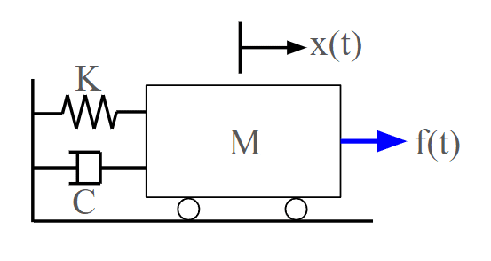
図1の運動方程式は次式となる。

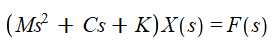
ラプラス変換をすると次式のようになる。
時間領域の変数が周波数領域の変数になるのと、部分部分が「s」となります。二階微分は「s^2」になっていますね。

X(s)が共通なので括ると次式のようになります。

入力F(s)に対する出力X(s)の形にすると次式のようになります。
これが入力に対する出力の伝達関数です。

ラプラス変換をするととても簡単に伝達関数を求められますね。
システムが大規模であったり、複雑であった場合に、システムをわかりやすく区切ってそれぞれの伝達関数を求めて、伝達関数にしてから連結すると単純な掛け算だけで求められたりします。
また、伝達関数の極（分母＝０になるsの値）や零点（分子＝０になるsの値）からおおよそのシステムの挙動を把握できる点も伝達関数にすることのメリットですね。

【English】

I am going to write this article as a "Toranomaki" of the minimum knowledge required (according to my own subjective judgment), remembering the control engineering classes I took in my university days. The reason I decided to write such an article is actually because recently I was given a homework assignment by one of my great professors, who told me to "Think about control properly!" I myself have reflected on my past self, who thought that I had to examine control more thoroughly and logically when manufacturing, but cut it off in moderation due to deadlines, and I would like to think about how I can connect the actual development with academic field.
To that end, I would like to begin by writing this article as a " Toranomaki" with very minimal content on the basics of the basics.

Laplace transform and transfer function

Simply put, the transfer function is obtained by Laplace transform using the following formula.

At that time in my university days, I only paid attention to the fact that a time-domain expression becomes a frequency-domain expression by Laplace transform. And as for the transfer function, at any rate, I did not think too much about it because I learned it in a control engineering class in my university, so I just assumed that it was somehow an expression of the system.
At this age, when I think about why we use Laplace transform again, I feel that it is useful for modeling large or complex systems, and I also feel that there are advantages such as the ease of calculating step response, impulse response, and various frequency responses by converting Laplace transform to transfer function. However, it may be difficult to realize its value unless you have an opportunity to model or analyze a large or complex system in the development field.

Laplace transform using Maple

Let's start with the Laplace transform using the Laplace transform command provided in Maple! The information presented here is in the Maple file attached at the end of this article, so if you have Maple, it will be easier to understand as you open it.

First, we write the initialization command "restart:", which means "initialize after reexecution" to prevent unintended variables from being set in memory and causing unintended results when the command is executed in Maple. Then, "with(inttrans):" is written to use the Laplace transform command. Now the Laplace transform can be executed with a single command.

To perform a Laplace transform in Maple, use the command "laplace(function of the time domain you want to transform, t, s)" The first argument is "the function of the time domain you want to transform". For example, "t" or "t^2". The second argument specifies the variable of the first argument. The third argument is the variable after Laplace transformation. Usually, it is "s". Now, let's calculate the Laplace transform in Maple, which is often used in control engineering.

The third one, "t^n" (t to the nth power), didn't turn out quite the way I was expecting, but the rest of the conversions are in the textbook form.

Now let's reverse the process and do an inverse Laplace transform. The commands are almost the same as for the Laplace transform. We use the command "invlaplace(function of the frequency domain to be transformed, s, t)." The only difference is that the "inv" is prefixed and the second and third arguments, "s" and "t," are reversed from those used for the Laplace transform. As with the Laplace transform, let's use Maple to compute the inverse Laplace transform, which is often used in control engineering.

As I thought, the inverse Laplace transform of the formula after the third expected transformation of the Laplace transform did not result in the expected "t^n". I may have to set up a more detailed transformation in this area. Other than that, the inverse Laplace transform was able to produce the expected form.

Example of a spring-mass damper system

Now that we know that the Laplace transform turns a time-domain function into a frequency-domain function, let's take a quick look at how it is used in control engineering. In control engineering, a system like the one shown in Figure 1 is studied by expressing it as a transfer function. The Laplace transform has the advantage of making it very easy to obtain the transfer function.

The motion equation in Figure 1 is as follows:

The Laplace transform yields the following equation. The variable in the time domain becomes the variable in the frequency domain and the partial part is "s". The second-order derivative is "s^2".

Since X(s) is common, it can be bracketed as follows:

In the form of output X(s) for input F(s), we obtain the transfer function.

It is very easy to find the transfer function by Laplace transform. If the system is large or complex, you can find the transfer function of each system by dividing the system into easily understandable parts and then concatenating them into a transfer function, which can be obtained by simple multiplication. Another advantage of transfer functions is that the approximate behavior of the system can be grasped from the poles (denominator = s value that becomes 0) and zeros (numerator = s value that becomes 0) of the transfer function.

【Sample】

Created by Maple 2023.2