詳説ディープラーニング（生成モデル編）が好評でしたので、付録としてTensorFlow 2.X による実装を紹介していきたいと思います（本文では PyTorch 1.X）。今回は、本文でも紹介したシンプルなオートエンコーダを実装していきます。

データローダ

本文では PyTorch で用意されているデータローダをそのまま使いましたが、TensorFlow では自前で用意する必要があります。そこで、PyTorch のデータローダとほぼ同じ挙動をするよう、下記のように実装しました（詳細な説明は割愛します）。

import numpy as np
import tensorflow as tf
from sklearn.utils import shuffle

class DataLoader(object):
    def __init__(self, dataset,
                 batch_size=100,
                 shuffle=False,
                 random_state=None):
        self.dataset = list(zip(dataset[0], dataset[1]))
        self.batch_size = batch_size
        self.shuffle = shuffle
        if random_state is None:
            random_state = np.random.RandomState(1234)
        self.random_state = random_state
        self._idx = 0
        self._reset()

    def __len__(self):
        N = len(self.dataset)
        b = self.batch_size
        return N // b + bool(N % b)

    def __iter__(self):
        return self

    def __next__(self):
        if self._idx >= len(self.dataset):
            self._reset()
            raise StopIteration()

        x, y = \
            zip(*self.dataset[self._idx:(self._idx + self.batch_size)])

        x = tf.convert_to_tensor(x)  # convert np.array to tf.Tensor
        y = tf.convert_to_tensor(y)

        self._idx += self.batch_size

        return x, y

    def _reset(self):
        if self.shuffle:
            self.dataset = shuffle(self.dataset,
                                   random_state=self.random_state)
        self._idx = 0

モデル

では、実際にモデルの定義〜学習・テストまでを行っていきましょう。本文と同じ構成で実装していきます。

まずは用いるライブラリからです。TF2 ではKerasレイヤーを用いることが前提となっています。

import os
import numpy as np
import tensorflow as tf
from tensorflow.keras import datasets
from tensorflow.keras.models import Model
from tensorflow.keras.layers import Dense
from tensorflow.keras import optimizers
from tensorflow.keras import metrics
from DataLoader import DataLoader  # 先ほど定義したデータローダ
import matplotlib
# matplotlib.use('Agg')
import matplotlib.pyplot as plt

続いて、モデルの定義です。PyTorchと違い、入力次元を定義しなくて良いかつ活性化関数を Dense 内で指定できるので、実装はかなりあっさりしています。

class Autoencoder(Model):
    def __init__(self):
        super().__init__()
        self.l1 = Dense(200, activation='relu')
        self.l2 = Dense(784, activation='sigmoid')

    def call(self, x):
        # encode
        h = self.l1(x)

        # decode
        y = self.l2(h)

        return y

では、実際に学習・テストを行っていきましょう。本文と同様、下記の構成で実装します。

if __name__ == '__main__':
    np.random.seed(1234)
    tf.random.set_seed(1234)

    '''
    1. Load data
    '''

    '''
    2. Build model
    '''

    '''
    3. Train model
    '''

    '''
    4. Test model
    '''

1. データ読み込み

先ほど定義した DataLoader インスタンスを用いてデータを用意します。

'''
1. Load data
'''
mnist = datasets.fashion_mnist
(x_train, y_train), (x_test, y_test) = mnist.load_data()
x_train = (x_train.reshape(-1, 784) / 255).astype(np.float32)
x_test = (x_test.reshape(-1, 784) / 255).astype(np.float32)

train_dataloader = DataLoader((x_train, y_train),
                              batch_size=100,
                              shuffle=True)
test_dataloader = DataLoader((x_test, y_test),
                             batch_size=1,
                             shuffle=False)

2. モデル構築

モデルインスタンスを生成するのみです。

'''
2. Build model
'''
model = Autoencoder()

3. モデルの学習

TensorFlow での勾配計算は tf.GradientTape を用います。また、 @tf.function を用いることで、関数を計算グラフオブジェクトに変換でき、処理が効率化されます。

'''
3. Train model
'''
criterion = tf.losses.BinaryCrossentropy()
optimizer = optimizers.Adam()

@tf.function
def compute_loss(x, preds):
    return criterion(x, preds)

@tf.function
def train_step(x):
    with tf.GradientTape() as tape:
        preds = model(x)
        loss = compute_loss(x, preds)
    grads = tape.gradient(loss, model.trainable_variables)
    optimizer.apply_gradients(zip(grads, model.trainable_variables))
    train_loss(loss)

train_loss = metrics.Mean()
epochs = 10

for epoch in range(epochs):

    for (x, _) in train_dataloader:
        train_step(x)

    print('Epoch: {}, Cost: {:.3f}'.format(
        epoch+1,
        train_loss.result()
    ))

4. テスト

学習後、本文同様にテストしてみます。

'''
4. Test model
'''
x, _ = next(iter(test_dataloader))
noise = tf.convert_to_tensor(
    np.random.binomial(1, 0.8, size=(x.numpy().shape)).astype(np.float32)
)
x_noise = x * noise

x_reconstructed = model(x_noise)

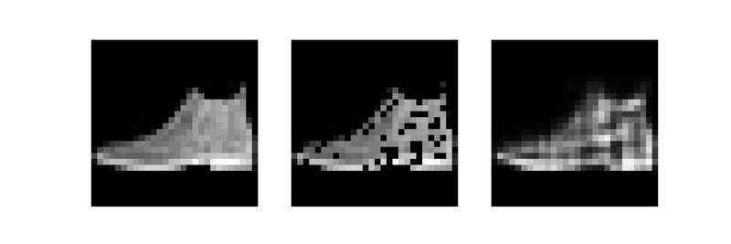
plt.figure(figsize=(18, 6))
for i, image in enumerate([x, x_noise, x_reconstructed]):
    image = image.numpy().reshape(28, 28)
    plt.subplot(1, 3, i+1)
    plt.imshow(image, cmap='binary_r')
    plt.axis('off')
plt.show()

この結果、下図のような結果が得られました。