【介入政策運営における構造変化🔥】『Japanese Foreign Exchange Interventions, 1971-2018:Estimating a Reaction Function Using the Best Proxy』:先行研究解説 No.13💝2023/11/01

Introduction:卒業論文は早めに仕上げたい💛
私もいよいよ卒業論文の執筆に
取りかかる時期がやって参りました👍
何事もアウトプット前提のインプットが
大事であると、noteで毎日発信してきました
これは、どのような内容で
あっても当てはまります👍
論文を一概に読んでも
記憶に残っていなかったり
大切な観点を忘れてしまっていたりしたら
卒業論文の進捗は滞ってしまうと思います
だからこそ、この「note」をフル活用して
卒業論文を1%でも
完成に向けて進めていきたいと思います
私の卒論執筆への軌跡を
どうぞご愛読ください📖
今回の参考文献🔥
今回、読み進めていく論文は
こちらのURLになります👍
『Japanese Foreign Exchange Interventions, 1971-2018: Estimating a Reaction Function Using the Best Proxy』
Takatoshi Ito(a), Tomoyoshi Yabu(b)
(a) School of International and Public Affairs, Columbia University, and GRIPS, Tokyo
(b) Department of Business and Commerce, Keio University
Japanese Foreign Exchange Interventions, 1971-2018: Estimating a Reaction Function Using the Best Proxy
December 12, 2019
Takatoshi Ito(a), Tomoyoshi Yabu(b)
(a) School of International and Public Affairs, Columbia University, and GRIPS, Tokyo
(b) Department of Business and Commerce, Keio University
前回のお復習い📝
5. Reaction Function
前回の投稿では、順序プロビットモデル(Ordered Probit Model)を用いて、通貨当局の反応関数を求めるプロセスについてアウトプットしました🌟
Ito and Yabu (2007)は、目標為替レートと介入のコスト関数をより現実的に定式化して、順序付けされたプロビットモデルとして反応関数を導出できるようにすることでモデルを拡張しました
Ito and Yabu (2007)の順序付けプロビットモデルを今一度お復習いとして確認しておくことにしましょう
$$
\\Ordered Probit Model \\ \\IInt_t = \begin{cases}
+1 &\text{if } \mu_2 < y_t^* \\
0 &\text{if } \mu_1 < y_t^* < \mu_2 \\ -1&\text{if } y_t^* < \mu_1 \cdots(2)
\end{cases} \\ \\ \\where y_t^*=X_t\beta +\epsilon_t \\with \epsilon_t \backsim i.i.d N(0,\sigma^2) and\\ \\X_t\beta=\beta_1(s_{t-1}-s_{t-2})+\beta_2(s_{t-1}-s_{t-1}^{MA})+\beta_3 IInt_{t-1}
$$
5.2. Structural Break Test
Before Ito and Yabu (2007), most papers estimated a model similar to the following:
Ito and Yabu (2007)より前は、ほとんどの論文が次のようなモデルを推定していました
$$
\\Structural Break Test\\ \\IInt_t =\varphi_0+\varphi_1(s_{t-1}-s_{t-2})\\ +\varphi_2(s_{t-1}-s_{t-1}^{MA})+\varphi_3 IInt_{t-1}+v_t (3)
$$
This model is considered to be a linearized version of Eq. (2). Note that φ1 < 0 when there is a lean-against-the wind intervention and φ2 < 0 when policy makers have a long-run target in mind; φ3 > 0 when there is a positive autocorrelation in interventions.
このモデルは、式(2):プロビットモデルの線形化バージョンであると考えられます
風に逆らう介入(lean-against-the wind intervention)がある場合は φ1< 0であり、政策立案者が為替レートの長期目標(long-run target)を念頭に置いている場合は φ2 < 0 であることに注意してください
またある月に介入が実施され、その次の月にも介入が実施される可能性が高くなっているという介入頻度に正の自己相関(positive autocorrelation in interventions)がある場合、φ3 > 0となります
Ito and Yabu (2007) analyzed the data from April 1991 to December 2002 to find that there was a structural break in the reaction function in June 1995 when Eisuke Sakakibara took charge of interventions.
Ito (2007) and Watanabe and Yabu (2013) asserted that when Zenbei Mizoguchi was in charge of the intervention from January 2003 to July 2004, the frequency and daily amount of intervention had a distinctive pattern—more frequent interventions of greater magnitude.
We take these observations as given and examine whether there exist any additional structural breaks between August 1971 and May 1995.
伊藤と藪(2007)は、1991年4月から2002年12月までのデータを分析し、榊原英資が財務省のトップとして介入政策の意思決定を担当した1995年6月に反応機能に構造的な断絶があったことを発見したのです💖
伊藤 (2007) と渡辺と藪 (2013) は、溝口善兵衛が2003年1月から 2004年7月まで介入政策の管理を担当していたとき、介入の頻度と1日あたりの量には独特のパターンがあり、より頻繁に、より大規模な介入が行われたと主張しました👀
この先行研究の筆者らはこれらの観察を所与のものとして受け取り、1971年8月から1995年5月までの間にさらなる構造的破壊が存在するかどうかを調査しているのです🌟
Here we analyze the data from August 1971 to May 1995 to conduct Andrews’ (1993) sup F test and search for an unknown structural break date.
The possible structural break dates are assumed to be the middle 70% of the sample period.
The first and last 15% of dates are excluded from break candidates. (We set the trimming parameter at 0.15).
The standard Chow test is conducted to obtain the F-statistic at each break candidate.
この先行研究では、1971年8月から1995年5月までのデータを分析して、Andrews (1993) の sup F テストを実施し、未知の構造変化の日を検索します
構造変化(structural break)の可能性がある日付は、サンプル期間の中央の70%であると想定されます
日付の最初と最後の 15% は、変化の日としての候補から除外されます
(トリミングパラメータ≒有意水準?を0.15に設定して検定していますね)
標準的なチョウ検定(The standard Chow test)は、各構造変化候補での F 統計量を取得するために実行されます💖
Fig. 5 shows the sequence of F-statistics for each break candidate. In the figure, the break dates are given on the horizontal axis and the Fstatistics on the vertical axis.
As shown, the F-statistic has the largest value in November 1981 at 4.80. This is larger than the 5% critical value of 4.09 but slightly lower than the 1% critical value of 5.12.
Therefore, we reject the null hypothesis of no break and accept the alternative of a structural break. In addition, based on the figure, the Fstatistic is single-peaked, implying that there are no other structural breaks.
The structural break date of November 1981 is a year and a half after a break date pointed out by Watanabe (1992) without conducting any structural break test.
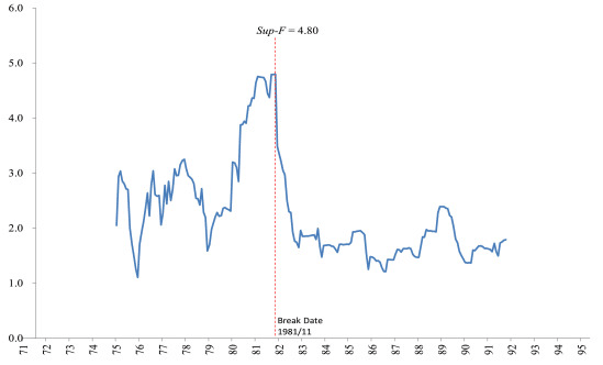
図5は、各ブレーク候補の F 統計量の順序を示しています。
この図では、横軸に構造変化の日(Break date)、縦軸にF統計量(F-statistics) が示されています
図5に示されているように1981年11月のF 統計量の値は、4.80と最大です
これは、有意水準5%の臨界値4.09よりも大きいですが、有意水準1%における臨界値の 5.12よりわずかに低くなっています
したがって、推計結果より「構造変化がないという帰無仮説H0」を棄却することになり、構造変化の代替手段(the alternative of a structural break)を受け容れることになります
さらに、この図に基づくと、F統計量(F-statistic) は単一ピークであり、他に構造的な変化がないことを示唆しています
1981年11月の構造変化の日(The structural break date of November 1981)は、渡辺(1992)が構造変化の検定を行わずに指摘した破壊日の1年半後のものであることがわかります
5.3. Conventional Regression
We split the full sample into five subperiods and estimate a linearized version of the reaction function Eq. (3) for each subsample.
As discussed in section 5.2, the sample before May 1995 is divided into two periods: 1) August 1971 to November 1981; and 2) December 1981 to May 1995 just before Eisuke Sakakibara took charge of interventions.
In addition, taking into account large-scale and frequent interventions by Zenbei Mizoguchi, the sample after June 1995 is divided into three periods: 3) June 1995 to December 2002; 4) January 2003 to July 2004; and 5) August 2004 to March 2018.
$$
\\Structural Break Test\\ \\IInt_t =\varphi_0+\varphi_1(s_{t-1}-s_{t-2})\\ +\varphi_2(s_{t-1}-s_{t-1}^{MA})+\varphi_3 IInt_{t-1}+v_t (3)
$$
この先行研究では、サンプル全体を5つのサブ期間に分割し、反応関数式(3)の線形化バージョンを推定しています📝
各サブサンプルについては、セクション 5.2 で説明したように、1995年5月より前のサンプルは2つの期間に分割されます
1) 1971年8月から1981年11月
2) 1981年12月から1995 年5月まで、榊原英資が介入を担当する直前の期間という分割になることを確認します
さらに、溝口善兵衛氏によって実施された大規模かつ頻繁な介入の期間を考慮すると、1995年6月以降のサンプルは、3つの期間に分かれています
3) 1995年6月から 2002年12月まで
4) 2003年1月~7月2004年
5) 2004年8月から2018 年3月まで
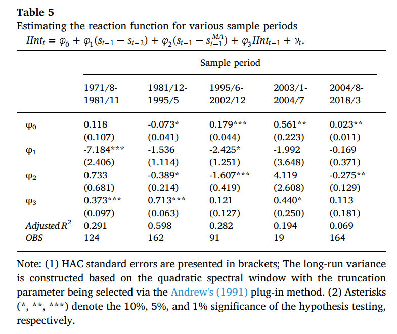
Table 5 summarizes the estimated results of Eq. (3) for each subsample. In the first period (August 1971 to November 1981), the parameter φ1 is significantly negative, but φ2 is not significantly different from zero.
The monetary authorities adopted a lean-against-the wind policy without setting any long-run targets.
They were only intent on reducing monthly volatility in the exchange rate. These results are consistent with the findings of Quirk (1977), Hutchison (1984), and Watanabe (1992).
On the other hand, the parameter φ3 is significantly positive and thus there was a positive autocorrelation in interventions. In the second period (December 1981 to May 1995), the parameter φ2 is significantly negative, but φ1 is not significantly different from zero.
That is, the monetary authorities had long-run targets in mind, but they were not mindful of reducing monthly volatility in the exchange rate.
These results are sharp contrast to the results of the first period but are consistent with the findings of Watanabe (1992).
The parameter φ3 has a large value of 0.713, a strong positive autocorrelation of interventions.
Adjusted R^2 has the largest value of 0.598 among the subsamples. Interventions were easiest to predict among the subsamples.

表5は、式(3)の推定結果をまとめたものです
$$
\\Structural Break Test\\ \\IInt_t =\varphi_0+\varphi_1(s_{t-1}-s_{t-2})\\ +\varphi_2(s_{t-1}-s_{t-1}^{MA})+\varphi_3 IInt_{t-1}+v_t (3)
$$
各サブサンプルについて以下の考察ができます
最初の期間 (1971年8月から1981年11 月) では、パラメータ φ1は大幅に負ですが、φ2はゼロから大きく変わりません
したがって、金融当局は長期的な目標を設定せず、風に逆らう政策(a lean-against-thewind policy)を採用したことになります
つまり、彼ら金融当局は為替レートの毎月の変動を減らすこと(reducing monthly volatility)だけを目的としていたのです
これらの結果は、Quirk (1977)、Hutchison (1984)、および渡辺 (1992) の発見と一致しています📝
一方、パラメーターφ3は統計的に有意に正であったことから、介入には正の自己相関があると解釈できます
なお、第2期 (1981 年12月から1995年5月) では、パラメータ φ2 は大幅に負ですが、φ1はゼロから大きく変わりません
つまり、金融当局は長期的な目標を念頭に置いていたのですが、為替レートの毎月の変動(ボラティリティ)を減らすことは念頭に置いていなかったのです
これらの結果は、第1期の結果とは顕著に対照的なものになりますが、Watanabe(1992) の結果と一致していることがわかったのです
そして、パラメータφ3は 0.713 という大きな値を持ち、介入の強い正の自己相関を示しています
なお、調整された決定係数(R^2)はサブサンプルの中で 0.598 という最大値を持っていることから、モデルの当てはまりの良さが見受けられます
そして、この期間における介入はサブサンプルの中で最も簡単に予測できたと言える結果になるでしょう
In the third period (June 1995 to December 2002), we obtain results similar to Ito and Yabu (2007), which analyzed the same period using daily data.
Both parameters of φ1 and φ2 are significantly negative. In other words, the monetary authorities paid attention to changes in the exchange rate as well as long-run targets.
In contrast to the results of the first and second periods, the parameter φ3 is now close to zero and no longer significant. There was no evidence of autocorrelation of interventions in this period.
Adjusted R^2 is smaller than it was in the previous two periods and thus interventions became more difficult to predict.
観察対象期間における第3期 (1995年6月から2002年12月) では、毎日のデータを使用して同期間を分析した伊藤と藪(2007)と同様の結果が得られます
この期間に対する推計結果において、φ1とφ2のパラメータは両方とも大幅に負です
言い換えれば、金融当局は長期目標だけでなく為替レートの変動にも注意を払っていたということがわかります
また第1期と第2期の結果とは対照的に、パラメータ φ3 はゼロに近くなり、もはや重要ではなくなりました
よって、この期間における介入の自己相関の証拠はないという解釈になります
また自由度修正済み決定係数(R^2)は、前の 2 つの期間よりも小さいため、介入の予測がより困難になった期間であるという解釈になります
In the fourth period (January 2003 to July 2004), the parameter φ3 is significantly positive, while both parameters φ1 and φ2 are not significantly different from zero.
The monetary authorities, thus, intervened only because they had intervened the month before.
As Ito (2007) and Watanabe and Yabu (2013) have pointed out, the monetary authorities may have had other motives to conduct interventions.
For the last period (August 2004 to March 2018), the parameter φ2 is significantly negative, while both parameters φ1 and φ3 are not significantly different from zero.
Therefore, the monetary authorities had long-run targets in mind but were not intent on reducing the volatility of the exchange rate. In addition, there was no positive autocorrelation of interventions.
Therefore, interventions during the previous month did not significantly increase the likelihood of interventions occurring during the following month.
Adjusted R2 has the smallest value of 0.069 among the subsamples because interventions took place during only 5 months of the 14-year period which also shows the difficulty of predicting interventions.
第4期 (2003年1月から2004年7月) では、介入実施における正の自己相関を示すパラメータφ3が有意に正である一方、パラメータφ1とφ2はいずれもゼロから大きく変わりません
したがって、金融当局が外国為替市場に介入したのは、単に前月に介入したからに過ぎないという解釈になります
伊藤 (2007) および渡辺と薮 (2013) が指摘したように、金融当局には介入を行う別の動機があった可能性があります📝
そして、最後の期間(2004年8月から2018年3月まで)では、パラメータφ2は大幅にマイナスですが、パラメータ φ1 と φ3 はどちらもゼロから大きく変わりません
したがって、金融当局は長期的な目標を念頭に置いていましたが、為替レートの変動(ボラティリティ)を軽減するつもりはありませんでした
さらに、介入の間に正の自己相関は見られませんでした
したがって、前月の介入は翌月に介入が発生する可能性を大幅に高めることはなかったと言えますね
なお介入は、14年間のわずか5か月の間に行われたため、自由度修正済み決定係数(R^2)はサブサンプルの中で最小値0.069となり、これはまた、モデルの当てはまりがあまり良くないこと、すなわち介入を予測することの難しさを示唆していると言えるでしょう
本日の解説は、ここまでとします
このような歴史や先行研究をしっかり理解した上で、卒業論文執筆に取り組んでいきたいです
読み終えた先行研究📚
『日本の為替介入の分析』 伊藤隆敏・著
経済研究 Vol.54 No.2 Apr. 2003
『Effects of the Bank of Japan’s intervention on yen/dollar exchange rate volatility』21 November 2004
Toshiaki Watanabe (a), Kimie Harada(b)
『The Effects of Japanese Foreign Exchange Intervention: GARCH Estimation and Change Point Detection』
Eric Hillebrand Gunther Schnabl Discussion
Paper No.6 October 2003
私の研究テーマについて🔖
私は「為替介入の実証分析」をテーマに
卒業論文を執筆しようと考えています📝
日本経済を考えたときに、為替レートによって
貿易取引や経常収支が変化したり
株や証券、債権といった金融資産の収益率が
変化したりと日本経済と為替レートとは
切っても切れない縁があるのです💝
(円💴だけに・・・)
経済ショックによって
為替レートが変化すると
その影響は私たちの生活に大きく影響します
だからこそ、為替レートの安定性を
担保するような為替介入はマクロ経済政策に
おいても非常に重要な意義を持っていると
推測しています
決して学部生が楽して執筆できる
簡単なテーマを選択しているわけでは無いと信じています
ただ、この卒業論文をやり切ることが
私の学生生活の集大成となることは事実なので
最後までコツコツと取り組んで参ります🔥
本日の解説は、以上とします📝
今後も経済学理論集ならびに
社会課題に対する経済学的視点による説明など
有意義な内容を発信できるように
努めてまいりますので
今後とも宜しくお願いします🥺
マガジンのご紹介🔔
こちらのマガジンにて
卒業論文執筆への軌跡
エッセンシャル経済学理論集、ならびに
【国際経済学🌏】の基礎理論をまとめています
今後、さらにコンテンツを拡充できるように努めて参りますので何卒よろしくお願い申し上げます📚
最後までご愛読いただき誠に有難うございました!
あくまで、私の見解や思ったことを
まとめさせていただいてますが
その点に関しまして、ご了承ください🙏
この投稿をみてくださった方が
ほんの小さな事でも学びがあった!
考え方の引き出しが増えた!
読書から学べることが多い!
などなど、プラスの収穫があったのであれば
大変嬉しく思いますし、投稿作成の冥利に尽きます!!
お気軽にコメント、いいね「スキ」💖
そして、お差し支えなければ
フォロー&シェアをお願いしたいです👍
今後とも何卒よろしくお願いいたします!
この記事が気に入ったらサポートをしてみませんか?