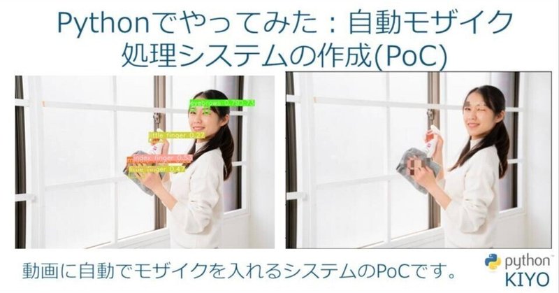
Pythonでやってみた16:自動モザイク処理システムの作成(PoC)

1.概要
今回は自動で画像や動画にモザイクをかけるシステムを作成していこうと思います。
練習用のため、対象は「眉毛」と「指」にしました。
1-1.実装フロー
実装は下記流れで進めていきたいと思います。
課題設定
何に対してモザイクをかけるか:今回は「眉毛」と「指」
目標値の設定:Accuracy(精度)、Recall(再現性)、Precision(適合性)
データ収集
ラベリング・アノテーション
モデルの選定・実装
データの前処理手法
物体検出モデル(例:YOLO、SSD、Faster R-CNN)の選択
モデルの学習
モザイク処理
テスト
展開・メンテナンス
2.データ収集
モザイクをかけるための学習データを集めます。今回は「静止画」と「動画」の2種類から取得していきます。
2-1.データ収集1:静止画
以前の記事で画像の自動取得方法やオープンソースを紹介しました。
今回はIcrawlerでサクッと適当に写真を自動取得しました。
[IN]
from icrawler.builtin import BaiduImageCrawler, BingImageCrawler, GoogleImageCrawler

keyword = '人の写真'
dir_root = 'Photo'
counts = 100 #取得枚数

def crawlImage(q=keyword, dir_root=dir_root, counts=counts):
    #フォルダがなければ作成
    if not os.path.exists(dir_root):
        os.makedirs(dir_root)

    crawler = BingImageCrawler(storage={'root_dir': dir_root})
    crawler.crawl(keyword=q, max_num=counts, filters=None)


crawlImage(q=keyword, dir_root=dir_root, counts=counts)

[OUT]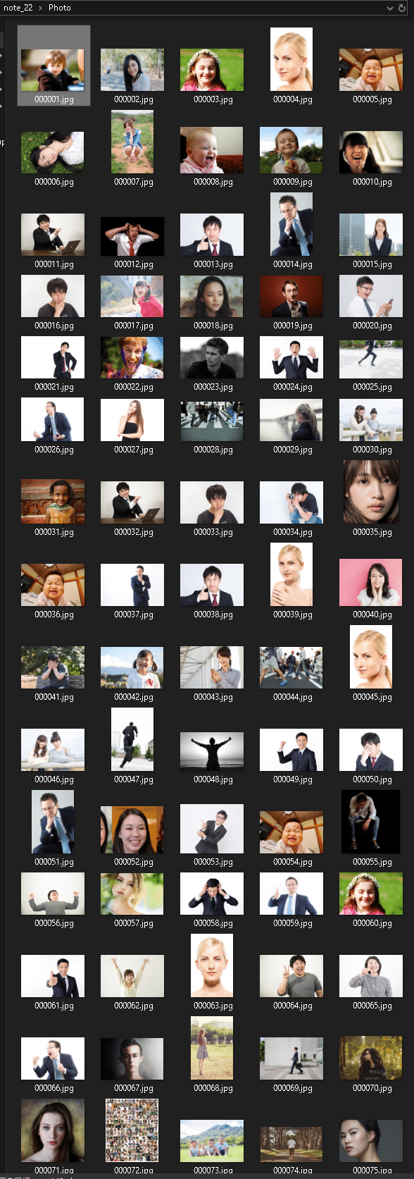
この中から手動で自分が欲しい画像を抽出しました。また、キーワードを変えながら何回か繰り返して画像を増やしました。
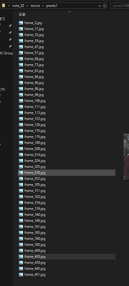
2-2.データ収集2:動画を分解
2-2-1.動画単体で処理
次に動画を静止画に分解して学習用データを抽出します。オリジナル素材があればよいですが、今回はフリー素材サイトから抽出しました。
videoAC:https://video-ac.com/
Pixabay:https://pixabay.com/ja/videos/
取得した動画から下記手順で静止画を取得しました。ライブラリはOpenCVを使用しており詳細は上記事の通りです。
手動で"movie"フォルダを事前に作成しておく
動画パスを取得し、OpenCVでインスタンス化
動画の総フレーム数を取得し、指定した割合で取得するフレーム数を計算
ランダムで動画から指定枚数の静止画をcv.imwiter()で抽出
[IN]
import cv2
import os

np.random.seed(123)

#.mp4 と .mov ファイルを検索
dir_root = 'movie'
path_movies = glob.glob(f'{dir_root}/*.mp4') + glob.glob(f'{dir_root}/*.mov')
path_movie = path_movies[0]

#フレーム数を取得
cap = cv2.VideoCapture(path_movie)
num_totalframes = cap.get(cv2.CAP_PROP_FRAME_COUNT)

#フレームを画像として保存
##保存用のフォルダ作成
_name = os.path.basename(path_movie).split('.')[0] #フォルダ用の名前を取得
_dir = f'{dir_root}/{_name}' #フォルダのPathを取得
if not os.path.exists(_dir):
    os.makedirs(_dir)
    print(f'{_dir}フォルダを作成')

ratio_getframe = 10 #総フレーム数の何%取得するか
num_frames = int(num_totalframes * ratio_getframe / 100) #取得するフレーム数
_num_random = np.random.randint(0, num_totalframes, size=num_frames) #ランダムにフレームを取得する
print(f'File:{os.path.basename(path_movie)}, 総フレーム数:{num_totalframes}, 取得フレーム数:{num_frames}')

for frame_number in _num_random:
    cap.set(cv2.CAP_PROP_POS_FRAMES, frame_number)
    ret, frame = cap.read()
    if ret:
        # フレームの保存
        cv2.imwrite(f"{_dir}/frame_{frame_number}.jpg", frame)

# リソースの解放
cap.release()

[OUT]
FileName:pexels1.mp4, 総フレーム数:469.0, 取得フレーム数:46
動画名を同じフォルダ名内に総フレーム数に対して指定した割合の静止画をランダムに抽出できました。
【別Ver.:枚数を指定】
動画が長尺になると割合で指定してもかなりの枚数になります。よって静止画数を指定するVersionも作成しました。
前回の"ratio_getframe(抽出するフレーム割合)"を削除し、num_framesを手打ちしただけとなります。
[IN]
import cv2
import os

np.random.seed(123)

#.mp4 と .mov ファイルを検索
dir_root = 'movie'
path_movies = glob.glob(f'{dir_root}/*.mp4') + glob.glob(f'{dir_root}/*.mov')
path_movie = path_movies[0]

#フレーム数を取得
cap = cv2.VideoCapture(path_movie)
num_totalframes = cap.get(cv2.CAP_PROP_FRAME_COUNT)

#フレームを画像として保存
##保存用のフォルダ作成
_name = os.path.basename(path_movie).split('.')[0] #フォルダ用の名前を取得
_dir = f'{dir_root}/{_name}' #フォルダのPathを取得
if not os.path.exists(_dir):
    os.makedirs(_dir)
    print(f'{_dir}フォルダを作成')

num_frames = 10 #取得するフレーム数
_num_random = np.random.randint(0, num_totalframes, size=num_frames) #ランダムにフレームを取得する
print(f'FileName:{os.path.basename(path_movie)}, 総フレーム数:{num_totalframes}, 取得フレーム数:{num_frames}')

for frame_number in _num_random:
    cap.set(cv2.CAP_PROP_POS_FRAMES, frame_number)
    ret, frame = cap.read()
    if ret:
        # フレームの保存
        cv2.imwrite(f"{_dir}/frame_{frame_number}.jpg", frame)

# リソースの解放
cap.release()

[OUT]
FileName:pexels1.mp4, 総フレーム数:469.0, 取得フレーム数:10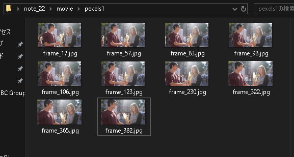
2-2-2.動画をまとめて処理
先の処理を指定した動画一括で処理できるように綺麗に関数化しました。今回は静止画枚数を指定して抽出しました。
[IN]
import cv2
import os

np.random.seed(123)

def getFrame_movie(path_movie:str, num_frames:int=None, ratio_frames:float=None):
    #フレーム数を取得
    cap = cv2.VideoCapture(path_movie)
    num_totalframes = cap.get(cv2.CAP_PROP_FRAME_COUNT)

    #フレームを画像として保存
    ##保存用のフォルダ作成
    _name = os.path.basename(path_movie).split('.')[0] #フォルダ用の名前を取得
    _dir = f'{dir_root}/{_name}' #フォルダのPathを取得
    if not os.path.exists(_dir):
        os.makedirs(_dir)
        print(f'{_dir}フォルダを作成')

    if ratio_frames is not None:
        num_frames = int(num_totalframes * ratio_frames / 100)
    nums_random = np.random.randint(0, num_totalframes, size=num_frames) #ランダムにフレームを取得する
    print(f'FileName:{os.path.basename(path_movie)}, 総フレーム数:{num_totalframes}, 取得フレーム数:{num_frames}')

    for frame_number in nums_random:
        cap.set(cv2.CAP_PROP_POS_FRAMES, frame_number)
        ret, frame = cap.read()
        if ret:
            # フレームの保存
            cv2.imwrite(f"{_dir}/frame_{frame_number}.jpg", frame)

    # リソースの解放
    cap.release()

#.mp4 と .mov ファイルを検索
dir_root = 'movie'
path_movies = glob.glob(f'{dir_root}/*.mp4') + glob.glob(f'{dir_root}/*.mov')
path_movie = path_movies[0]

for dir_movie in path_movies:
    getFrame_movie(path_movie=dir_movie, num_frames=10) #取得枚数を指定
# getFrame_movie(path_movie=dir_movie, ratio_frames=8) #総フレーム数の何%取得するか指定[OUT]
FileName:pexels1.mp4, 総フレーム数:469.0, 取得フレーム数:10
movie/pexels2フォルダを作成
FileName:pexels2.mp4, 総フレーム数:244.0, 取得フレーム数:10
movie/pixabay1フォルダを作成
FileName:pixabay1.mp4, 総フレーム数:251.0, 取得フレーム数:10
movie/pixabay2フォルダを作成
FileName:pixabay2.mp4, 総フレーム数:848.0, 取得フレーム数:10
movie/pixabay3フォルダを作成
FileName:pixabay3.mp4, 総フレーム数:614.0, 取得フレーム数:10
movie/videoac1フォルダを作成
FileName:videoac1.mov, 総フレーム数:468.0, 取得フレーム数:10
movie/videoac2フォルダを作成
FileName:videoac2.mov, 総フレーム数:1130.0, 取得フレーム数:10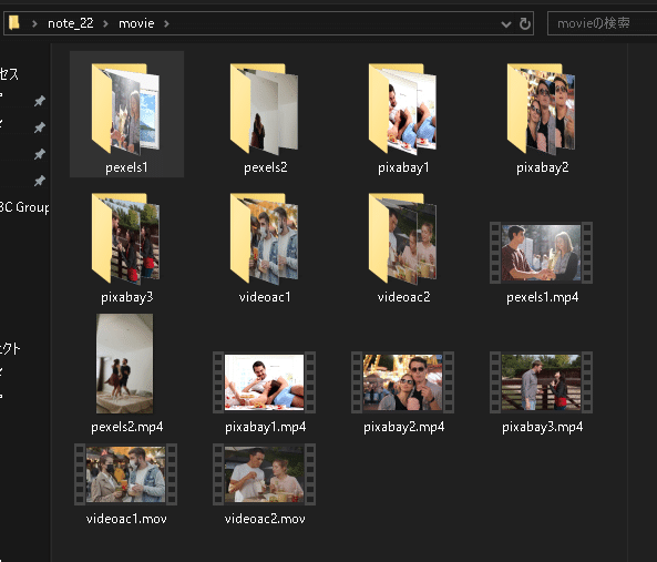
3.ラベリング・アノテーション
YOLOv5のような物体検出をするためには機械学習の正解値(ラベル名と座標)がわかるようにアノテーションが必要になります。今回はアノテーションツールとしてVOTTを使用しました。詳細は下記記事の通りです。概要のみ抜粋しました。
3-1.ラベル付け
今回は欲しいラベル名を下記の通り作成しました。
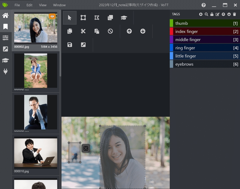
アノテーションが性能に影響を及ぼすみたいなので、できる限り丁寧にラベルを作成していきます。
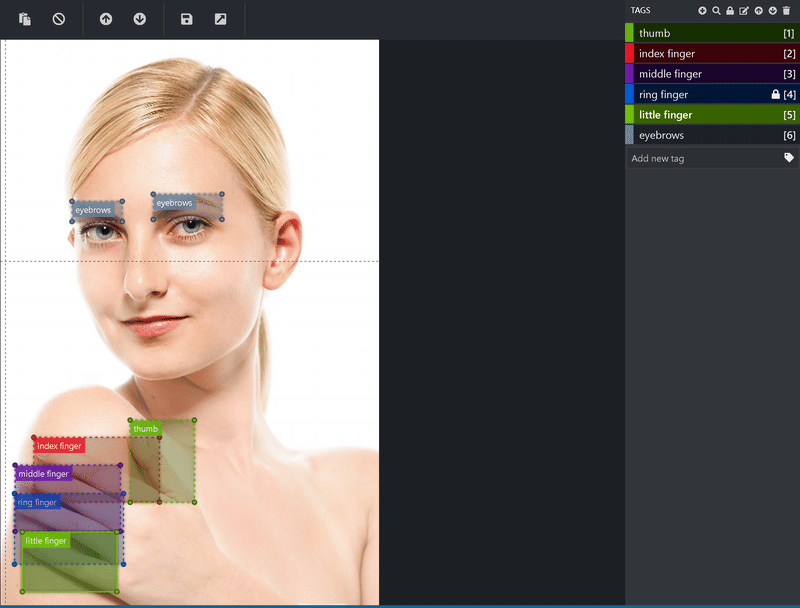
アノテーションの結果は下記の通りです。
3-2.結果(JSON)の出力
「プロジェクトの保存」を押した後に「プロジェクトをエクスポート」を押すことでexportフォルダとjsonファイルが出力されました。
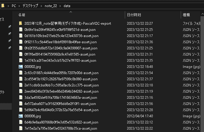
念のために生成されたアノテーションデータがあるjsonファイルと画像ファイルの数が同じか確認しました。
[IN]
pd.options.display.max_rows = 100
paths_img = glob.glob(f'data/*.jpg')
paths_json = glob.glob(f'data/*.json')
print(f'画像枚数:{len(paths_img)}, json枚数:{len(paths_json)}')
infos_json = {'name':[], 'path':[]}
for path_json in paths_json:
with open(path_json) as f:
data = json.load(f)
_name = data['asset']['name'] #アノテーションした画像ファイル名
infos_json['name'].append(_name)
infos_json['path'].append(path_json)
_df1 = pd.DataFrame([os.path.basename(_) for _ in paths_img])
_df2 = pd.DataFrame(infos_json).sort_values('name').reset_index(drop=True)
_df = pd.concat([_df1, _df2], axis=1)
_df.columns = ['img', 'name', 'path']
_df
[OUT]
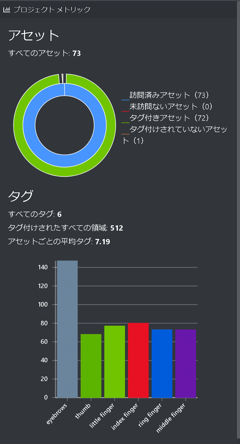
画像枚数:71, json枚数:71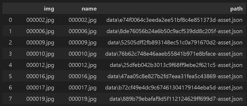
3-3.ラベルの作成
前記事の通り、タグと座標情報は"region"キーのtags, boundingBox, pointsに含まれます。 1個目のJSONファイルを確認すると、自分で作成したアノテーションの情報が含まれることを確認できます。
[IN]
paths_json = glob.glob(f'data/*.json')
path_json = paths_json[0]
with open(path_json) as f:
    data = json.load(f)

for region in data['regions']:
    # Bounding Boxの値を取得
    left = region["boundingBox"]["left"]
    top = region["boundingBox"]["top"]
    width = region["boundingBox"]["width"]
    height = region["boundingBox"]["height"]
    # Pointsの値を取得
    x_LU, y_LU = region["points"][0]["x"], region["points"][0]["y"]
    x_RU, y_RU = region["points"][1]["x"], region["points"][1]["y"]
    x_RB, y_RB = region["points"][2]["x"], region["points"][2]["y"]
    x_LB, y_LB = region["points"][3]["x"], region["points"][3]["y"]

    # 小数点一桁で表示
    print(f'tag: {region["tags"]}, Bounding Box: {{left: {left:.1f}, top: {top:.1f}, width: {width:.1f}, height: {height:.1f}}}, Points: {{LU: ({x_LU:.1f}, {y_LU:.1f}), RU: ({x_RU:.1f}, {y_RU:.1f}), RB: ({x_RB:.1f}, {y_RB:.1f}), LB: ({x_LB:.1f}, {y_LB:.1f})}}')


[OUT]
tag: ['eyebrows'], Bounding Box: {left: 542.7, top: 153.8, width: 39.5, height: 9.3}, Points: {LU: (542.7, 153.8), RU: (582.3, 153.8), RB: (582.3, 163.1), LB: (542.7, 163.1)}
tag: ['eyebrows'], Bounding Box: {left: 605.5, top: 148.5, width: 48.5, height: 13.6}, Points: {LU: (605.5, 148.5), RU: (654.0, 148.5), RB: (654.0, 162.1), LB: (605.5, 162.1)}
tag: ['little finger'], Bounding Box: {left: 323.8, top: 192.0, width: 25.2, height: 43.9}, Points: {LU: (323.8, 192.0), RU: (349.0, 192.0), RB: (349.0, 235.9), LB: (323.8, 235.9)}
ラベル自体は数が多くないため手動で作成しました。
[IN]
#手動で作成したタグ
tags = {'thumb':0, 'index':1, 'middle':2, 'ring':3, 'little':4, 'eyebrows':5}

[OUT]
-
3-4.絶対座標を相対座標に変換
前記事の通り(関数名は変更)、下記を実施しました。
タグ(TAGS)を数値に変換するための辞書作成(今回は手動)
絶対座標を相対座標に変換
得られるリスト情報を文字列(str)に変換
テキスト(拡張子.txt)にラベル情報を記載
[IN]
from typing import List, Dict, Tuple, Union

if not os.path.exists('labels'):
    os.makedirs('labels')
    print('labelsフォルダを作成')

#手動で作成したタグ
dict_tag2id = {'thumb':0, 'index finger':1, 'middle finger':2, 'ring finger':3, 'little finger':4, 'eyebrows':5}

#アノテーションの座標を絶対値から相対値に変換
def coordinate_abs2rel(annot_data:Dict, height, width, left, top):
    width_img, height_img = annot_data['asset']['size']['width'], annot_data['asset']['size']['height'] #画像のサイズ

    #座標の絶対値を計算
    x_move, y_move = width/2, height/2 #画像の中心を取得
    x_abs = left + x_move #x座標:絶対値
    y_abs = top + y_move #y座標:絶対値
    #座標を相対比に変換
    x_center = x_abs/width_img #x座標:相対値
    y_center = y_abs/height_img #y座標:相対値
    height_rel = height/height_img #高さ:相対値
    width_rel = width/width_img #幅:相対値
    return [x_center, y_center, height_rel, width_rel]

#リストを文字列(Str)に変換
def convert_list2str(data):
    data = str(data)
    data = data.replace('[', '')
    data = data.replace(']', '')
    data = data.replace(',', '')
    return data


#データ処理
paths_json = glob.glob(f'data/*.json')
for path_json in tqdm(paths_json):
    #jsonファイルを読み込み
    with open(path_json) as f:
        data = json.load(f)

    regions = data['regions'] #アノテーション情報を取得
    filename_img = data['asset']['name'].split('.')[0] #画像のファイル名を取得
    text = '' #出力用の文字列

    for idx, region in enumerate(regions):
        tagname = region['tags'][0] #タグ情報を取得
        tag = dict_tag2id[tagname] #タグIDを取得
        keys_coord = ['height', 'width', 'left', 'top'] #座標情報のキー
        height, width, left, top = [region['boundingBox'][key] for key in keys_coord] #座標を取得
        data_coord = coordinate_abs2rel(data, height, width, left, top)
        labelinfo = [tag] + data_coord #タグIDと座標を結合
        textdata = convert_list2str(labelinfo) #タグIDと座標を文字列に変換
        if not idx == len(regions) - 1:
            text += textdata + '\n' #タグIDと座標を改行で結合
        else:
            text += textdata #最後の行は改行しない

    #テキストファイルを保存
    with open(f'labels/{filename_img}.txt', 'w') as f:
        f.write(text) #出力用のテキストをファイルに書き込む

[OUT]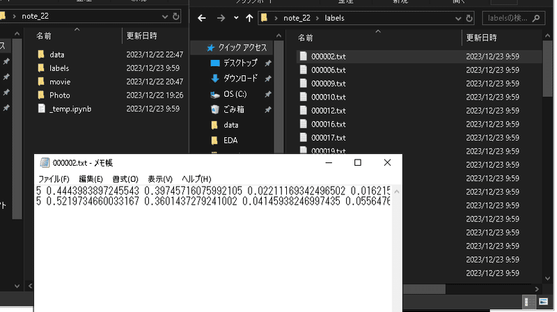
4.機械学習
4-1.モデルの選定
今回は過去に実施したことがあるという理由でYOLOv5を選定しました。YOLOは比較的早いスパンで最新モデルが出るため、必要に応じて最適なモデルを選定したらよいと思います。
環境構築は事前に対応済みとして、次節に進みます。
[Terminal]
git clone https://github.com/ultralytics/yolov5
cd yolov5
pip install -r requirements.txt
4-2.データセット/data.yamlの準備
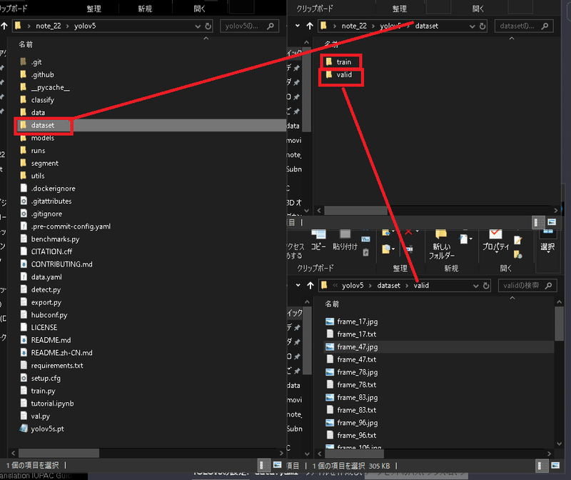
まずは学習用(Train)、検証用(valid)、テスト用(test)に画像とラベルを振り分けます。今回はデータ数が少ないためTrain/Validのみで使用します。
環境構築時にクローンしたレポジトリ:yolov5内にdatasetフォルダを作成し、その中に"train"と"valid"フォルダを作成し、画像とラベルを移動させました(ファイルの選択方法がランダムのため、特に画像・ラベルをランダムに振り分けるコードは作成しておりません)。
次にデータセットのパス、クラス名、クラス数などを定義するYamlファイルを作成しました。
[data.yaml]
train: C:/Users/KIYO/Desktop/note_22/yolov5/dataset/train  # トレーニングデータのパス
val: C:/Users/KIYO/Desktop/note_22/yolov5/dataset/valid      # 検証データのパス

nc: 6 # クラスの数
names: ['thumb', 'index finger', 'middle finger', 'ring finger', 'little finger', 'eyebrows']  # クラスの名前
4-3.モデルの学習
モデル学習時はterminalの作業位置を"train.py"があるフォルダ(デフォルト:yolov5)に移動して下記コードを実行します。
[Terminal]
python train.py --batch <バッチ数> --epochs <エポック数> --data <data.yamlのパス>
今回は下記で実行しました。私のPC(RTX 2060 SUPER)だと50epochs:20min、200epoch:1h23minくらいで完了しました。結果でいうとbatch:5、epochs:50は指は検出できず、eyebrowsの検出精度も低かったです。
[Terminal※低性能]
python train.py --batch 5 --epochs 50 --data data.yaml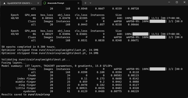
[Terminal]
python train.py --batch 20 --epochs 200 --data data.yaml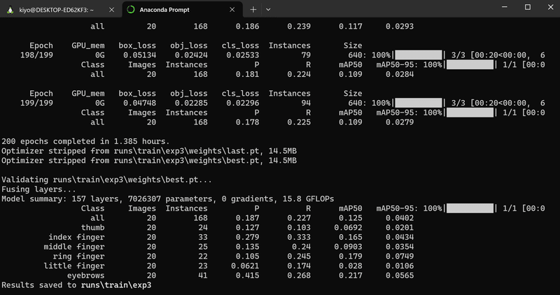
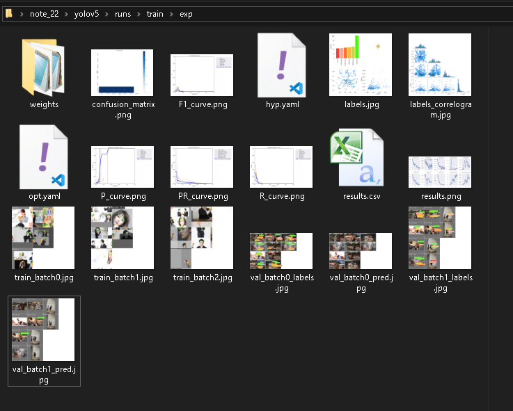
学習が完了するとTerminalに記載の通り下記結果が出力されました。
” runs\train\exp”:学習結果
” runs\train\exp\weights”:学習結果の重み
4-4.結果の検証
学習した重みを使用して物体検出を実施します。重みの指定は"--weight"、データのディレクトリは"--source"オプションを使用します。
[Terminal]
python detect.py --weight <学習した重みファイルのパス>

[Terminal:学習用データも指定]
python detect.py --source<データのディレクトリ>  --weight <学習した重みファイルのパス>
本当はテストデータを使用するのが正しいですが、今回はデータ数がないため学習に使用したTrain/Validを使用して確認しました。
[Terminal:学習]
python detect.py --source "C:/Users/KIYO/Desktop/note_22/yolov5/dataset/train" --weights "C:/Users/KIYO/Desktop/note_22/yolov5/runs/train/exp/weights/best.pt"[Terminal:検証]
python detect.py --source "C:/Users/KIYO/Desktop/note_22/yolov5/dataset/valid" --weights "C:/Users/KIYO/Desktop/note_22/yolov5/runs/train/exp/weights/best.pt"学習済みデータを使用しているためテストでどうなるか不明ですが、現状では物体検出がうまくいくことを確認できました。
[IN]
import random

#学習(Train)データ
paths_img = glob.glob('yolov5/runs/detect/exp6/*.jpg')
paths_img = paths_img[1:5]
random.shuffle(paths_img) #縦長の画像の配列がいまいちなのでシャッフル

#可視化
fig, axs = plt.subplots(2, 2, figsize=(10, 6))
for idx_row in range(2):
    for idx_col in range(2):
        path_img = paths_img[idx_row*2 + idx_col]
        img_bgr = cv2.imread(path_img)
        img_rgb = cv2.cvtColor(img_bgr, cv2.COLOR_BGR2RGB)
        axs[idx_row, idx_col].imshow(img_rgb)
        axs[idx_row, idx_col].axis('off')

[OUT]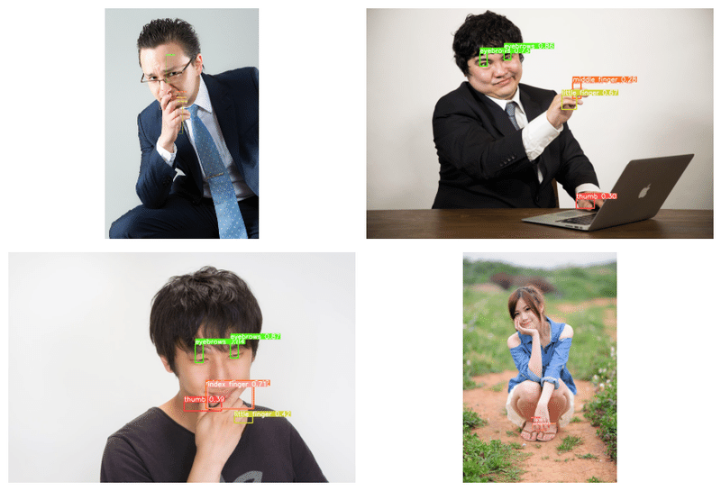
[IN]
#検証(Valid)データ
paths_img = glob.glob('yolov5/runs/detect/exp7/*.jpg')
paths_img = paths_img[1:5]
#可視化
fig, axs = plt.subplots(2, 2, figsize=(10, 6))
for idx_row in range(2):
    for idx_col in range(2):
        path_img = paths_img[idx_row*2 + idx_col]
        img_bgr = cv2.imread(path_img)
        img_rgb = cv2.cvtColor(img_bgr, cv2.COLOR_BGR2RGB)
        axs[idx_row, idx_col].imshow(img_rgb)
        axs[idx_row, idx_col].axis('off')

plt.tight_layout()
plt.show()

[OUT]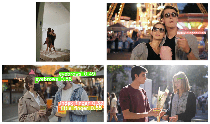
5.モザイク処理
次に物体認識をした箇所にモザイクをかけるためのクラスを作成します。内容は以前の記事を参考にしました。
サンプル画像として、ぱくたそのフリー素材を使用しました。
5-1.おさらい:モザイク処理
モザイク処理はOpenCVの機能を利用して処理することが可能です。サンプルコードは下記の通りであり、下記機能を追加しました。
モザイク(画像の縮小->元に戻す)、ぼかし、ガウシアンフィルタを追加
モザイク処理後に、指定したピクセル範囲を塗りつぶすメソッドも追加
トリミングや画像情報取得のメソッド追加
[IN]
from PIL import Image
import cv2
import glob

class MosaicProcessor:
    def __init__(self, path:str):
        self.img_bgr = cv2.imread(path)  # インスタンス変数として定義
        self.img_rgb = cv2.cvtColor(self.img_bgr, cv2.COLOR_BGR2RGB)  # BGR->RGB

    def mosaic_img(self, img_cv2=None, ratio:int=10):
        if img_cv2 is None:
            img_cv2 = self.img_rgb

        h, w, _ = img_cv2.shape #画像の高さ、幅、チャンネル数
        img_small = cv2.resize(img_cv2, (w//ratio, h//ratio)) #画像を縮小
        img_mosaic = cv2.resize(img_small, (w, h), interpolation=cv2.INTER_AREA) #元のサイズに拡大
        return img_mosaic

    def gaussianBlur(self, img_cv2=None, kernel:tuple=(15, 15), sigma:float=0.0):
        if img_cv2 is None:
            img_cv2 = self.img_rgb
        img_gaussianblur = cv2.GaussianBlur(img_cv2, kernel, sigma) #kernelは正の奇数
        return img_gaussianblur

    def blur_img(self, img_cv2=None, kernel:tuple=(10, 10)):
        if img_cv2 is None:
            img_cv2 = self.img_rgb
        img_blur = cv2.blur(img_cv2, kernel) #
        return img_blur

    #きついモザイク処理用
    def mosaic_Adv_img(self, img_cv2=None, ratio:int=10, pixel_size:int=10):
        if img_cv2 is None:
            img_cv2 = self.img_rgb

        h, w, _ = img_cv2.shape  # 画像の高さ、幅、チャンネル数
        img_small = cv2.resize(img_cv2, (w//ratio, h//ratio))  # 画像を縮小
        img_mosaic = cv2.resize(img_small, (w, h), interpolation=cv2.INTER_AREA)  # 元のサイズに拡大

        # 指定したピクセル範囲を、ピクセルの左上の色で埋める
        for i in range(0, h, pixel_size):
            for j in range(0, w, pixel_size):
                img_mosaic[i:i+pixel_size, j:j+pixel_size] = img_mosaic[i, j]

        return img_mosaic

    def trim_img(self, img_cv2=None, x:int=0, y:int=0, w:int=100, h:int=100):
        if img_cv2 is None:
            img_cv2 = self.img_rgb
        img_trim = img_cv2[y:y+h, x:x+w]
        return img_trim

    def show_property(self):
        print(f'Path Name: {path_img}')
        print('width: {}, height: {}, channel: {}'.format(self.img_rgb.shape[1], self.img_rgb.shape[0], self.img_rgb.shape[2]))
        print('dtype: {}'.format(self.img_rgb.dtype))
[IN]
# 検証
paths_img = glob.glob('photo/*')
path_img = paths_img[0]
mosaic = MosaicProcessor(path_img)
#可視化
fig, axs = plt.subplots(2, 3, figsize=(10, 6))
axs[0, 0].imshow(mosaic.img_rgb)
axs[0, 0].set_title('オリジナル画像(処理前)')
axs[0, 1].imshow(mosaic.mosaic_img(ratio=10))
axs[0, 1].set_title(f'モザイク処理(縮小比率: 10)')
axs[0, 2].imshow(mosaic.mosaic_Adv_img(ratio=10, pixel_size=10))
axs[0, 2].set_title(f'モザイク処理_Adv(縮小比率: 10, pixel_size: 10)')
axs[1, 0].imshow(mosaic.gaussianBlur(kernel=(15, 15), sigma=10))
axs[1, 0].set_title(f'ガウシアンフィルタ(kernel: 15, sigma: 10)')
axs[1, 1].imshow(mosaic.blur_img(kernel=(15, 15)))
axs[1, 1].set_title(f'ぼかしフィルタ(kernel: 15)')
axs[1, 2].imshow(mosaic.trim_img(x=500, y=100, w=300, h=300))
axs[1, 2].set_title(f'トリミング(x: 500, y: 100, w: 300, h: 300)')
plt.tight_layout()
plt.show()

[OUT]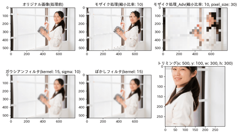
5-2.画像へ物体検出を適用
次に学習済みモデルを使用して物体検出+座標取得をし、得られた画像にモザイクをかける処理をします。今回はPytorch Hubを利用してモデルを利用しました。環境構築やPytorch Hubは下記記事に記載しております。
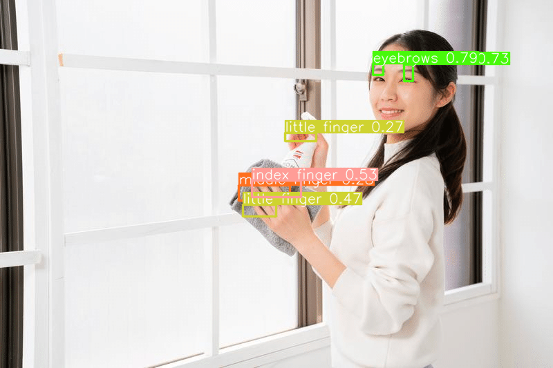
5-2ー1.モデルの動作確認
学習済みモデルの重みを利用してYolov5を使用して座標、信頼度、クラスを取得しました。問題なく動作することを確認できました。
[IN]
import torch

path_modelweight = 'yolov5/runs/train/exp3/weights/last.pt'
model = torch.hub.load('ultralytics/yolov5', 'custom', path_modelweight)

paths_img = glob.glob('photo/*')
path_img = paths_img[0]

results = model(path_img)
print(results)
print(results.pred[0])
display(results.pandas().xyxy[0])
results.show()[OUT]
Using cache foundin C:\Users\KIYO/.cache\torch\hub\ultralytics_yolov5_master
YOLOv5 2023-12-23 Python-3.10.13 torch-2.1.2+cpu CPU
Fusing layers...
Model summary: 157 layers, 7026307 parameters, 0 gradients, 15.8 GFLOPs
Adding AutoShape...
image 1/1: 533x800 1 index finger, 1 middle finger, 2 little fingers, 2 eyebrowss
Speed: 4.0ms pre-process, 69.0ms inference, 1.0ms NMS per image at shape (1, 3, 448, 640)
tensor([[5.39440e+02, 9.26340e+01, 5.54249e+02, 1.08078e+02, 7.88765e-01, 5.00000e+00],
[5.84219e+02, 9.37218e+01, 5.97983e+02, 1.17127e+02, 7.28395e-01, 5.00000e+00],
[3.64180e+02, 2.61138e+02, 4.35419e+02, 2.85584e+02, 5.34127e-01, 1.00000e+00],
[3.51804e+02, 2.96935e+02, 3.99344e+02, 3.13394e+02, 4.74042e-01, 4.00000e+00],
[3.45571e+02, 2.68360e+02, 4.19587e+02, 2.90879e+02, 2.77449e-01, 2.00000e+00],
[4.12747e+02, 1.92203e+02, 4.57668e+02, 2.04836e+02, 2.67182e-01, 4.00000e+00]])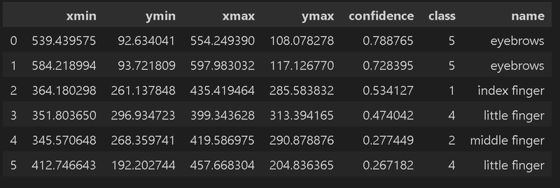
5-2ー2.モザイク処理の実装
下記の通り実装しました。
%matplotlib inlineを追加して、画像がJupyterで表示されるようにする
前節のモザイクclassを流量して処理器を作成
BoundingBoxは小数値だが画像範囲は整数のため、画像の幅・高さを計算する時点で整数に変換しておく(小数点差によるズレ防止)
YOLOv5で得られる結果はx,y座標の絶対値のため、処理に合わせて計算
モザイクclassがオリジナルデータをインスタンス変数として保持しているためそこに上書き(classのインスタンスが保持する画像のオリジナル情報は上書きされる)
[IN]
%matplotlib inline
from PIL import Image
import cv2
import glob

class MosaicProcessor:
    def __init__(self, path:str):
        self.img_bgr = cv2.imread(path)  # インスタンス変数として定義
        self.img_rgb = cv2.cvtColor(self.img_bgr, cv2.COLOR_BGR2RGB)  # BGR->RGB

    def mosaic_img(self, img_cv2=None, ratio:int=10):
        if img_cv2 is None:
            img_cv2 = self.img_rgb

        h, w, _ = img_cv2.shape
        img_small = cv2.resize(img_cv2, (w//ratio, h//ratio))
        img_mosaic = cv2.resize(img_small, (w, h), interpolation=cv2.INTER_AREA)
        return img_mosaic

    def gaussianBlur(self, img_cv2=None, kernel:tuple=(15, 15), sigma:float=0.0):
        if img_cv2 is None:
            img_cv2 = self.img_rgb
        img_gaussianblur = cv2.GaussianBlur(img_cv2, kernel, sigma) #kernelは正の奇数
        return img_gaussianblur

    def blur_img(self, img_cv2=None, kernel:tuple=(10, 10)):
        if img_cv2 is None:
            img_cv2 = self.img_rgb
        img_blur = cv2.blur(img_cv2, kernel) #
        return img_blur

    #きついモザイク処理用
    def mosaic_Adv_img(self, img_cv2=None, ratio:int=10, pixel_size:int=10):
        if img_cv2 is None:
            img_cv2 = self.img_rgb

        h, w, _ = img_cv2.shape  # 画像の高さ、幅、チャンネル数
        img_small = cv2.resize(img_cv2, (w//ratio, h//ratio))  # 画像を縮小
        img_mosaic = cv2.resize(img_small, (w, h), interpolation=cv2.INTER_AREA)  # 元のサイズに拡大

        # 指定したピクセル範囲を、ピクセルの左上の色で埋める
        for i in range(0, h, pixel_size):
            for j in range(0, w, pixel_size):
                img_mosaic[i:i+pixel_size, j:j+pixel_size] = img_mosaic[i, j]

        return img_mosaic

    def trim_img(self, img_cv2=None, x:int=0, y:int=0, w:int=100, h:int=100):
        if img_cv2 is None:
            img_cv2 = self.img_rgb
        img_trim = img_cv2[y:y+h, x:x+w]
        return img_trim

    def show_property(self):
        print(f'Path Name: {path_img}')
        print('width: {}, height: {}, channel: {}'.format(self.img_rgb.shape[1], self.img_rgb.shape[0], self.img_rgb.shape[2]))
        print('dtype: {}'.format(self.img_rgb.dtype))


import torch
#学習済みモデルによるYOLOV5のインスタンス化
path_modelweight = 'yolov5/runs/train/exp3/weights/last.pt'
model = torch.hub.load('ultralytics/yolov5', 'custom', path_modelweight)

#画像取得
paths_img = glob.glob('photo/*')
path_img = paths_img[0]
#推論
results = model(path_img)
#検出結果
detections = results.pred[0] #(x1, y1, x2, y2, confidense, class)の順でリスト化されている
#モザイク処理器のインスタンス化
mosaic = MosaicProcessor(path_img)

#処理
for det in detections:
    x1, y1, x2, y2, conf, class_id = det
    width_det, height_det = int(x2) - int(x1), int(y2) - int(y1) #小数点以下を切り捨て:数値のズレを防止
    img_trim = mosaic.trim_img(x=int(x1), y=int(y1), w=int(width_det), h=int(height_det))
    img_mosaic = mosaic.mosaic_img(img_trim, ratio=10)
    # トリミングされた領域のサイズに合わせてモザイク処理された画像を調整
    mosaic.img_rgb[int(y1):int(y2), int(x1):int(x2)] = img_mosaic


plt.imshow(mosaic.img_rgb)
plt.show()

[OUT]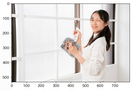
参考までに別の画像でも処理しました。奥の指は認識できていますが、手前のピントが合っていない部分はモデルは認識できておりません。
6.実装:動画へ適用
今までは学習済みモデルを使用して静止画にモザイク処理を適用しました。次は同じ要領で動画に適用させます。
動画は静止画(フレーム)の集まりであるため、動画をフレームごとに分割し、各フレームに対して物体検出とモザイク処理を行い、処理済みのフレームを再び動画として結合することで実装できると想定されます。処理は引き続きOpenCVを利用していきます。
動画はPixabayとvideoACから、認識しやすそうなやつを選定しました。
6-1.コードの修正:class MosaicProcessor_CV2
OpenCVの処理ではcv2.VideoCapture()でキャプチャーした動画をcap.read()でBGRのarrayで出力します。現状のモザイク処理classは画像のpathで受け入れるようにしているため、これをarrayで処理できるように変更します。
基本的に動画は各フレームごとでarrayが出力されるため下記のように修正しました。
インスタンス化時は何も渡さない
画像(フレーム)は適宜reset_imgメソッドで追加する
その他は全て同じ
[IN]
%matplotlib inline
import torch
from PIL import Image
import cv2
import glob

class MosaicProcessor_CV2:
    def __init__(self):
        self.img_bgr = None
        self.img_rgb = None

    def reset_img(self, frame_img:np.ndarray):
        self.img_bgr = frame_img
        self.img_rgb = cv2.cvtColor(frame_img, cv2.COLOR_BGR2RGB)

    def mosaic_img(self, img_cv2=None, ratio:int=10):
        if img_cv2 is None:
            img_cv2 = self.img_rgb

        h, w, _ = img_cv2.shape
        img_small = cv2.resize(img_cv2, (w//ratio, h//ratio))
        img_mosaic = cv2.resize(img_small, (w, h), interpolation=cv2.INTER_AREA)
        return img_mosaic

    def gaussianBlur(self, img_cv2=None, kernel:tuple=(15, 15), sigma:float=0.0):
        if img_cv2 is None:
            img_cv2 = self.img_rgb
        img_gaussianblur = cv2.GaussianBlur(img_cv2, kernel, sigma) #kernelは正の奇数
        return img_gaussianblur

    def blur_img(self, img_cv2=None, kernel:tuple=(10, 10)):
        if img_cv2 is None:
            img_cv2 = self.img_rgb
        img_blur = cv2.blur(img_cv2, kernel) #
        return img_blur

    #きついモザイク処理用
    def mosaic_Adv_img(self, img_cv2=None, ratio:int=10, pixel_size:int=10):
        if img_cv2 is None:
            img_cv2 = self.img_rgb

        h, w, _ = img_cv2.shape  # 画像の高さ、幅、チャンネル数
        img_small = cv2.resize(img_cv2, (w//ratio, h//ratio))  # 画像を縮小
        img_mosaic = cv2.resize(img_small, (w, h), interpolation=cv2.INTER_AREA)  # 元のサイズに拡大

        # 指定したピクセル範囲を、ピクセルの左上の色で埋める
        for i in range(0, h, pixel_size):
            for j in range(0, w, pixel_size):
                img_mosaic[i:i+pixel_size, j:j+pixel_size] = img_mosaic[i, j]

        return img_mosaic

    def trim_img(self, img_cv2=None, x:int=0, y:int=0, w:int=100, h:int=100):
        if img_cv2 is None:
            img_cv2 = self.img_rgb
        img_trim = img_cv2[y:y+h, x:x+w]
        return img_trim

    def show_property(self):
        print(f'Path Name: {path_img}')
        print('width: {}, height: {}, channel: {}'.format(self.img_rgb.shape[1], self.img_rgb.shape[0], self.img_rgb.shape[2]))
        print('dtype: {}'.format(self.img_rgb.dtype))
本classで画像Pathでなく配列を渡しても、同様に問題なく処理できることを確認できました。
[IN]
import torch
#学習済みモデルによるYOLOV5のインスタンス化
path_modelweight = 'yolov5/runs/train/exp3/weights/last.pt'
model = torch.hub.load('ultralytics/yolov5', 'custom', path_modelweight)

#画像取得
paths_img = glob.glob('photo/*')
path_img = paths_img[0]
array_img = cv2.imread(path_img)

#推論
results = model(path_img)
#検出結果
detections = results.pred[0] #(x1, y1, x2, y2, confidense, class)の順でリスト化されている
#モザイク処理器のインスタンス化
mosaic = MosaicProcessor_CV2()
mosaic.reset_img(array_img)

#処理
for det in detections:
    x1, y1, x2, y2, conf, class_id = det
    width_det, height_det = int(x2) - int(x1), int(y2) - int(y1) #小数点以下を切り捨て:数値のズレを防止
    img_trim = mosaic.trim_img(x=int(x1), y=int(y1), w=int(width_det), h=int(height_det))
    img_mosaic = mosaic.mosaic_img(img_trim, ratio=10)
    # トリミングされた領域のサイズに合わせてモザイク処理された画像を調整
    mosaic.img_rgb[int(y1):int(y2), int(x1):int(x2)] = img_mosaic

plt.imshow(mosaic.img_rgb)
plt.show()

[OUT]
6-2.動画読込:cv2.VideoCapture、
動画の読み込み"cv2.VideoCapture(<動画のパス>)"を使用します。動画の情報を取得することが出来ました。
[IN]
#処理動画
path_movie2 = 'movie/videoac1.mov'

#動画の読み込み
cap = cv2.VideoCapture(path_movie2)
width, height, fps = cap.get(cv2.CAP_PROP_FRAME_WIDTH), cap.get(cv2.CAP_PROP_FRAME_HEIGHT), cap.get(cv2.CAP_PROP_FPS)
print(f'width: {width}, height: {height}, fps: {fps}')

[OUT]
width: 640.0, height: 360.0, fps: 50.0
6-3.フレーム処理:cv2.VideoWriter
フレーム処理は”cv2.VideoWriter()”で実施します。フレーム処理に使用するコーデックは(*'DIVX')を使用しました。
下記を実行するとcv2.VideoWriter()に記載したファイル名のファイルが作成されます。この時点ではメディアプレイヤーで開いてもレンダリングできないエラーが出ますので無視しても問題ありません。
[IN]
fourcc = cv2.VideoWriter_fourcc(*'DIVX')
out = cv2.VideoWriter('output1.mp4', fourcc, fps, (int(width), int(height))) #出力動画の設定

[OUT]
6-4.フレーム取得:cap.read()
フレームの取得はcap.read()で実施できます。frameはBGRのarrayであるため、モザイク処理クラスのインスタンスに渡せば処理できます。
[IN]
#初期化
mosaic = MosaicProcessor_CV2()

# フレームごとの処理
while cap.isOpened():
    ret, frame = cap.read()
    if not ret:
        break

[OUT]
6-4.モザイク処理
今までやってきたことを下記の通り実装しました。
モザイククラスをインスタンス化:mosaic
cap.read()でフレーム取得
学習済みモデルにframe(静止画のarray)を渡して物体検出
mosaicインスタンスにframeを渡して初期化
物体検出の出力から座標情報をmosaicに渡して処理
out.writeでフレームの書き出し
リソースの解放
[IN]
#初期化
mosaic = MosaicProcessor_CV2()

# フレームごとの処理
while cap.isOpened():
    ret, frame = cap.read()
    if not ret:
        break

    # YOLOv5で物体検出
    results = model(frame) # 推論
    detections = results.pred[0] # (x1, y1, x2, y2, confidense, class)の順でリスト化されている

    mosaic.reset_img(frame) # フレームのリセット

    # モザイク処理
    for det in detections:
        x1, y1, x2, y2, conf, class_id = det
        width_det, height_det = int(x2) - int(x1), int(y2) - int(y1)
        img_trim = mosaic.trim_img(x=int(x1), y=int(y1), w=int(width_det), h=int(height_det))
        ratio_mosaic  = 10 # モザイクの粗さ設定

        img_trim = mosaic.trim_img(x=int(x1), y=int(y1), w=int(width_det), h=int(height_det))
        #サイズが小さすぎるとエラーになるためtry文
        try:
            img_mosaic = mosaic.mosaic_img(img_trim, ratio=ratio_mosaic)
        except Exception as e:
            print(e)
            ratio_mosaic_small = ratio_mosaic // 3
            img_mosaic = mosaic.mosaic_img(img_trim, ratio=ratio_mosaic_small)

        mosaic.img_bgr[int(y1):int(y2), int(x1):int(x2)] = cv2.cvtColor(img_mosaic, cv2.COLOR_RGB2BGR)


    # 処理済みフレームの書き出し
    out.write(mosaic.img_bgr)

# リソースの解放
cap.release()
out.release()
[OUT]
6-5.完成コード
完成したコードをひとまとめにしました。ベースとしては下記を正しく設定したら動作すると思います。
学習済みモデルの重み:path_modelweight
動画のパス:path_movie
OpenCVのコーデック(※Windowsは*'DIVX'のままでOKと思います)
[IN]
%matplotlib inline
import torch
from PIL import Image
import cv2
import glob

class MosaicProcessor_CV2:
    def __init__(self):
        self.img_bgr = None
        self.img_rgb = None

    def reset_img(self, frame_img:np.ndarray):
        self.img_bgr = frame_img
        self.img_rgb = cv2.cvtColor(frame_img, cv2.COLOR_BGR2RGB)

    def mosaic_img(self, img_cv2=None, ratio:int=10):
        if img_cv2 is None:
            img_cv2 = self.img_rgb

        h, w, _ = img_cv2.shape
        img_small = cv2.resize(img_cv2, (w//ratio, h//ratio))
        img_mosaic = cv2.resize(img_small, (w, h), interpolation=cv2.INTER_AREA)
        return img_mosaic

    def gaussianBlur(self, img_cv2=None, kernel:tuple=(15, 15), sigma:float=0.0):
        if img_cv2 is None:
            img_cv2 = self.img_rgb
        img_gaussianblur = cv2.GaussianBlur(img_cv2, kernel, sigma) #kernelは正の奇数
        return img_gaussianblur

    def blur_img(self, img_cv2=None, kernel:tuple=(10, 10)):
        if img_cv2 is None:
            img_cv2 = self.img_rgb
        img_blur = cv2.blur(img_cv2, kernel) #
        return img_blur

    #きついモザイク処理用
    def mosaic_Adv_img(self, img_cv2=None, ratio:int=10, pixel_size:int=10):
        if img_cv2 is None:
            img_cv2 = self.img_rgb

        h, w, _ = img_cv2.shape  # 画像の高さ、幅、チャンネル数
        img_small = cv2.resize(img_cv2, (w//ratio, h//ratio))  # 画像を縮小
        img_mosaic = cv2.resize(img_small, (w, h), interpolation=cv2.INTER_AREA)  # 元のサイズに拡大

        # 指定したピクセル範囲を、ピクセルの左上の色で埋める
        for i in range(0, h, pixel_size):
            for j in range(0, w, pixel_size):
                img_mosaic[i:i+pixel_size, j:j+pixel_size] = img_mosaic[i, j]

        return img_mosaic

    def trim_img(self, img_cv2=None, x:int=0, y:int=0, w:int=100, h:int=100):
        if img_cv2 is None:
            img_cv2 = self.img_rgb
        img_trim = img_cv2[y:y+h, x:x+w]
        return img_trim

    def show_property(self):
        print(f'Path Name: {path_img}')
        print('width: {}, height: {}, channel: {}'.format(self.img_rgb.shape[1], self.img_rgb.shape[0], self.img_rgb.shape[2]))
        print('dtype: {}'.format(self.img_rgb.dtype))


#学習済みモデルによるYOLOV5のインスタンス化
path_modelweight = 'yolov5/runs/train/exp3/weights/last.pt'
model = torch.hub.load('ultralytics/yolov5', 'custom', path_modelweight)

#処理動画
path_movie = 'movie/videoac1.mov'

#動画の読み込み
cap = cv2.VideoCapture(path_movie)
width, height, fps = cap.get(cv2.CAP_PROP_FRAME_WIDTH), cap.get(cv2.CAP_PROP_FRAME_HEIGHT), cap.get(cv2.CAP_PROP_FPS)
print(f'width: {width}, height: {height}, fps: {fps}')

#出力動画の設定:https://fourcc.org/codecs.php
fourcc = cv2.VideoWriter_fourcc(*'DIVX')
out = cv2.VideoWriter('output1.mp4', fourcc, fps, (int(width), int(height))) #出力動画の設定

#初期化
mosaic = MosaicProcessor_CV2()

# フレームごとの処理
while cap.isOpened():
    ret, frame = cap.read()
    if not ret:
        break

    # YOLOv5で物体検出
    results = model(frame) # 推論
    detections = results.pred[0] # (x1, y1, x2, y2, confidense, class)の順でリスト化されている

    mosaic.reset_img(frame) # フレームのリセット

    # モザイク処理
    for det in detections:
        x1, y1, x2, y2, conf, class_id = det
        width_det, height_det = int(x2) - int(x1), int(y2) - int(y1)
        img_trim = mosaic.trim_img(x=int(x1), y=int(y1), w=int(width_det), h=int(height_det))
        ratio_mosaic  = 10 # モザイクの粗さ設定

        img_trim = mosaic.trim_img(x=int(x1), y=int(y1), w=int(width_det), h=int(height_det))
        #サイズが小さすぎるとエラーになるためtry文
        try:
            img_mosaic = mosaic.mosaic_img(img_trim, ratio=ratio_mosaic)
        except Exception as e:
            print(e)
            ratio_mosaic_small = ratio_mosaic // 3
            img_mosaic = mosaic.mosaic_img(img_trim, ratio=ratio_mosaic_small)

        mosaic.img_bgr[int(y1):int(y2), int(x1):int(x2)] = cv2.cvtColor(img_mosaic, cv2.COLOR_RGB2BGR)


    # 処理済みフレームの書き出し
    out.write(mosaic.img_bgr)

# リソースの解放
cap.release()
out.release()

[OUT]
1つ目の動画は処理できていることが分かるくらいには処理できていますが、結構漏れが多いです。
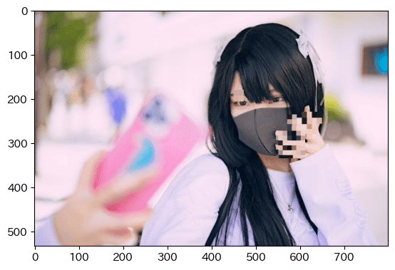
2個目の動画は「眉毛」と「指」ともにかなり精度が悪いです。おそらく眉毛は、学習時のデータセットにサングラスの人がいなかったためと思います。指に関して、何でこんなに精度が悪いかは不明です・・・・

7.所感
所感としては「なんとなくできそうなことは分かったけど実用レベルには工夫が必要」と感じました。
まず精度に関して、今回学習に使用したデータ数はTrain:51、valid:20です。たったこのくらいのデータ数で検証結果が出たのであれば御の字だと思います。
労力に関して、データ数を増やそうとするとアノテーションが重要になりますが、やはりこれは非常に手間のためどうしても工数が発生してしまうのは辛いところです。アノテーションのBoundingBoxは綺麗につけないと精度が下がる恐れがあるため、注意が必要です。
モデルに関して、YOLOは最新モデルも出ているためこれらを使用すれば改善はできると思います。
よって、最新モデルでデータを増やせば結構いいところまで行けるような気はしました。
参考資料
あとがき
次はセマンティックセグメンテーション(U-net)でできるか検証
この記事が気に入ったらサポートをしてみませんか?