mixturesbパッケージは（1次元の）混合正規分布まわりの計算、特に

・乱数生成
・確率密度関数の計算
・対数尤度関数の計算
・EMアルゴリズムによる最尤推定およびクラスタリング

をサポートするR言語のプライベートパッケージです。主に混合正規分布の理解の助けになるパッケージを提供したいという思いから、株式会社すうがくぶんかの教材のひとつとして作成しました。

なお、このパッケージの作成にあたってはtidyverse styleを尊重するよう心掛けています。将来的には混合分布全般の乱数生成やEM-algorithm、Bayes推定（WAICなどを含む）の理解を助ける関数を提供できることが目標です。

1. Installation

mixturesbパッケージは、devtoolsパッケージのinstall_github関数を用いてインストールすることができます。

# Let's install and load our package !
devtools::install_github("utaka233/mixturesb")
library(mixturesb)

2. 混合正規分布の乱数生成とEM-algorithm

2.1 問題設定
母平均が-2.0, 母標準偏差が3.0の正規分布N(-2.0, 3.0²)と母平均が1.0, 母標準偏差が4.0の正規分布N(1.0, 4.0²)を0.25 : 0.75の比率で混合した分布（混合正規分布）を考えます。

このような母集団からサイズ100の標本を抽出し、抽出した標本からEM-algorithmを用いて母集団パラメータ（母平均・母標準偏差・混合比率）を推定してみましょう。

2.2 乱数生成
まず標本抽出（要するに乱数生成）は次のように行うことが出来ます。

# Random numbers generation from 1-dim. mixtures of normal distribution.
library(dplyr)
library(ggplot2)
x <- random_mixt_normal(n = 100, mu = c(-2.0, 1.0), sigma = c(3.0, 4.0), ratio = c(0.25, 0.75))
data <- tibble(x = x)
data
#> # A tibble: 100 x 1
#>         x
#>     <dbl>
#>  1  -1.31
#>  2   1.71
#>  3   1.96
#>  4  10.0 
#>  5   5.71
#>  6   3.29
#>  7   9.22
#>  8   2.46
#>  9  -3.10
#> 10   6.65
##  ... with 90 more rows
ggplot(data = data, mapping = aes(x = x)) + geom_histogram(binwidth = 2.0)

2.3 EM-algorithm
このようにして抽出した標本に対して、EM-algorithmを用いた最尤推定を行ってみましょう。

# EM-algorithm
result_em <- x %>%
    EM_mixt_normal(max_iter = 100,    # 更新の最大繰り返し数
                   tol = 0.01,    # 対数尤度のtolerance
                   init_mu = c(-1.0, 1.0),    # 母平均の初期値
                   init_sigma = c(1.0, 1.0),    # 母標準偏差の初期値
                   init_ratio = c(0.5, 0.5))    # 混合比率の初期値
summary(result_em)    # 推定結果の概要
#> * Numbers of Components:
#>              num_components
#> component_1:             22
#> component_2:             78
#> 
#> * Parameters of Components:
#>                     mu    sigma     ratio
#> component_1: -1.731535 3.075150 0.3189233
#> component_2:  2.283424 2.906745 0.6810767
#> 
#> log_likelihood            AIC            BIC     iterations 
#>      -267.1272       544.2544       557.2803        13.0000 

2.4 EM-algorithmの更新履歴
EM-algorithmの更新ごとの対数尤度は、tibbleまたはグラフで確認することが出来ます。

# tibble : history of EM-algorithm
result_em$log_likelihood_history    # 対数尤度の更新履歴のtibble
#> # A tibble: 14 x 2
#>     iter log_likelihood
#>    <int>          <dbl>
#>  1     0          -576.
#>  2     1          -270.
#>  3     2          -268.
#>  4     3          -268.
#>  5     4          -268.
#>  6     5          -267.
#>  7     6          -267.
#>  8     7          -267.
#>  9     8          -267.
#> 10     9          -267.
#> 11    10          -267.
#> 12    11          -267.
#> 13    12          -267.
#> 14    13          -267.
plot_LL(result_em)    # visualization with ggplot2

2.5 EM-algorithmの推定結果
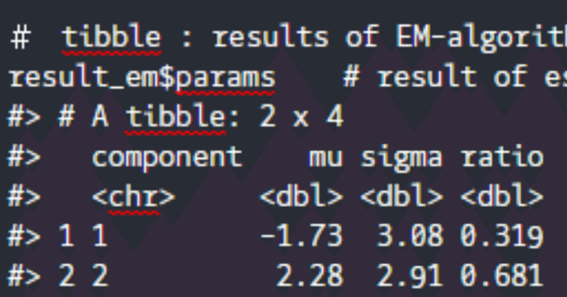
EM-algorithmによるパラメータ推定の結果や各データポイントがどのcomponentに所属していると推定されたかはtibbleで取得できます。また、ヒストグラム上にcomponentを可視化できます。

＃　tibble : results of EM-algorithm
result_em$params    # result of estimated parameters
#> # A tibble: 2 x 4
#>   component    mu sigma ratio
#>   <chr>     <dbl> <dbl> <dbl>
#> 1 1         -1.73  3.08 0.319
#> 2 2          2.28  2.91 0.681
result_em$estimated_component    # result of esimated component
#> # A tibble: 100 x 2
#>         x estimated_component
#>     <dbl> <chr>              
#>  1  -1.31 component2         
#>  2   1.71 component2         
#>  3   1.96 component2         
#>  4  10.0  component2         
#>  5   5.71 component2         
#>  6   3.29 component2         
#>  7   9.22 component2         
#>  8   2.46 component2         
#>  9  -3.10 component1         
#> 10   6.65 component2         
#> # ... with 90 more rows
plot_components(result_em, binwidth = 1.0)    # visualization with ggplot2

2.6 未知のデータに対する所属componentの予測
未知のデータが新たに母集団から得られたとき、そのデータがどのcomponentに所属しているかを予測できます。

# Predict component for new data.
x <- -5:5    # new data
predict(result_em, x)    # prediction for x

3. より発展的な使い方：アニメーション

mixturesbパッケージは、EM-algorithmによる最尤推定の更新履歴をアニメーションで提供します。以下のスクリプトを実行すると、初期パラメータから収束までの更新の様子をgif形式のファイルで生成し、作業ディレクトリに書き出します。

＃ Animation with gif file
plot_history(result_em)

4. おわりに

最後までお読みいただき有難うございました。R package作成における個人的な目標は、統計学の理解に資するパッケージをつくることです。mixturesbパッケージも、より充実させて色々な人の統計学の勉強の傍らにいるパッケージにできればなぁと思っています。

将来的にはCRANから配布できればと思っています。mixturesbパッケージをご愛顧していただけますよう、どうかよろしくお願いいたします。