次にニューラルネットワークについての勾配を求めます。前回は関数に対するものでした。

簡単なニューラルネットワークを例にして実際に勾配を求めましょう！GoogleDriveをマウントしてから以下を記述していきます。

import sys, os
sys.path.append('/content/drive/My Drive/deep-learning-from-scratch')
import numpy as np
from common.functions import softmax, cross_entropy_error
from common.gradient import numerical_gradient

class simpleNet:
   def __init__(self):
       self.W = np.random.randn(2,3)
   def predict(self, x):
       return np.dot(x, self.W)
   def loss(self, x, t):
       z = self.predict(x)
       y = softmax(z)
       loss = cross_entropy_error(y, t)
       return loss

simpleNetというクラスを定義します。

必要なデータを取り込んでいます。

from common.functions import softmax, cross_entropy_error
from common.gradient import numerical_gradient

simpleNetを使っていきます。

net = simpleNet()
print(net.W)

重みパラメーターの出力です。

[[ 1.17708788 1.58646892 -1.8613983 ]
[ 0.57469687 1.72680926 -0.75397319]]

x = np.array([0.6, 0.9])
p = net.predict(x)
print(p)

推論結果です。

[-0.4296473 0.44853191 1.20995208]

np.argmax(p)

最大値のインデックス

2

tには正解ラベルを入力して計算します。

t = np.array([0,0,1])
net.loss(x,t)

0.3843789075215526

これらを使い勾配を求めます。

まず損失関数です。

f = lambda w: net.loss(x, t)

勾配を求める式numerical_gradient(f,x)に損失関数fを使います。

dW = numerical_gradient(f, net.W)
print(dW)

[[ 0.07010028 0.16868719 -0.23878747]
[ 0.10515043 0.25303078 -0.35818121]]

2層のニューラルネットワークを一つのクラスとして実装します。

import sys, os
sys.path.append('/content/drive/My Drive/deep-learning-from-scratch')
from common.functions import *
from common.gradient import numerical_gradient

class TwoLayerNet:
   def __init__(self, input_size, hidden_size, output_size, weight_init_std=0.01):
       # 重みの初期化
       self.params = {}
       self.params['W1'] = weight_init_std * np.random.randn(input_size, hidden_size)
       self.params['b1'] = np.zeros(hidden_size)
       self.params['W2'] = weight_init_std * np.random.randn(hidden_size, output_size)
       self.params['b2'] = np.zeros(output_size)
   
　　def predict(self, x):
       W1, W2 = self.params['W1'], self.params['W2']
       b1, b2 = self.params['b1'], self.params['b2']
   
       a1 = np.dot(x, W1) + b1
       z1 = sigmoid(a1)
       a2 = np.dot(z1, W2) + b2
       y = softmax(a2)
       
       return y
       
   # x:入力データ, t:教師データ
   def loss(self, x, t):
       y = self.predict(x)
       
       return cross_entropy_error(y, t)
   
   def accuracy(self, x, t):
       y = self.predict(x)
       y = np.argmax(y, axis=1)
       t = np.argmax(t, axis=1)
       
       accuracy = np.sum(y == t) / float(x.shape[0])
       return accuracy
       
   # x:入力データ, t:教師データ
   def numerical_gradient(self, x, t):
       loss_W = lambda W: self.loss(x, t)
       
       grads = {}
       grads['W1'] = numerical_gradient(loss_W, self.params['W1'])
       grads['b1'] = numerical_gradient(loss_W, self.params['b1'])
       grads['W2'] = numerical_gradient(loss_W, self.params['W2'])
       grads['b2'] = numerical_gradient(loss_W, self.params['b2'])
       
       return grads
       
   def gradient(self, x, t):　　
       W1, W2 = self.params['W1'], self.params['W2']
       b1, b2 = self.params['b1'], self.params['b2']
       grads = {}
       
       batch_num = x.shape[0]
       
       # forward
       a1 = np.dot(x, W1) + b1
       z1 = sigmoid(a1)
       a2 = np.dot(z1, W2) + b2
       y = softmax(a2)
       
       # backward
       dy = (y - t) / batch_num
       grads['W2'] = np.dot(z1.T, dy)
       grads['b2'] = np.sum(dy, axis=0)
       
       dz1 = np.dot(dy, W2.T)
       da1 = sigmoid_grad(a1) * dz1
       grads['W1'] = np.dot(x.T, da1)
       grads['b1'] = np.sum(da1, axis=0)
       return grads

テストデータで評価します。TwoLayerNetクラスを使ってMINISTデータセットを使って学習、テストデータで評価します。

import sys, os
sys.path.append('/content/drive/My Drive/deep-learning-from-scratch')
import numpy as np
import matplotlib.pyplot as plt
from dataset.mnist import load_mnist

# データの読み込み
(x_train, t_train), (x_test, t_test) = load_mnist(normalize=True, one_hot_label=True)

network = TwoLayerNet(input_size=784, hidden_size=50, output_size=10)

iters_num = 10000  # 繰り返しの回数を適宜設定する

train_size = x_train.shape[0]
batch_size = 100
learning_rate = 0.1
train_loss_list = []
train_acc_list = []
test_acc_list = []
iter_per_epoch = max(train_size / batch_size, 1)

for i in range(iters_num):
   batch_mask = np.random.choice(train_size, batch_size)
   x_batch = x_train[batch_mask]
   t_batch = t_train[batch_mask]
   
   # 勾配の計算
   #grad = network.numerical_gradient(x_batch, t_batch)
   grad = network.gradient(x_batch, t_batch) 　#高速版
   
   # パラメータの更新
   for key in ('W1', 'b1', 'W2', 'b2'):
       network.params[key] -= learning_rate * grad[key]
   
   loss = network.loss(x_batch, t_batch)
   train_loss_list.append(loss)
   
   if i % iter_per_epoch == 0:
       train_acc = network.accuracy(x_train, t_train)
       test_acc = network.accuracy(x_test, t_test)
       train_acc_list.append(train_acc)
       test_acc_list.append(test_acc)
       print("train acc, test acc | " + str(train_acc) + ", " + str(test_acc))

# グラフの描画
markers = {'train': 'o', 'test': 's'}
x = np.arange(len(train_acc_list))
plt.plot(x, train_acc_list, label='train acc')
plt.plot(x, test_acc_list, label='test acc', linestyle='--')
plt.xlabel("epochs")
plt.ylabel("accuracy")
plt.ylim(0, 1.0)
plt.legend(loc='lower right')
plt.show()

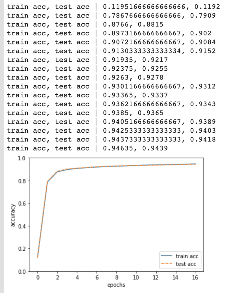
認識精度が上がっていくのが確認できますね。